Results

This page separates deterministic synthetic examples from real market-data examples. The plots are committed artifacts generated by the notebook clients, so the documentation build stays deterministic and does not depend on live notebook execution or market-data downloads.

Machine-readable copies of the comparison tables are committed under results/:

• results/synthetic_comparison.csv

• results/real_data_comparison.csv

• results/generated_comparison_summary.csv

• results/generated_repeatability_trials.csv

• results/real_data_method_comparison.csv

• results/larger_real_data_comparison.csv

• results/ansatz_comparison.csv

For repeatable synthetic benchmark summaries, regenerate a compact comparison CSV with:

python scripts/generate_comparison_results.py

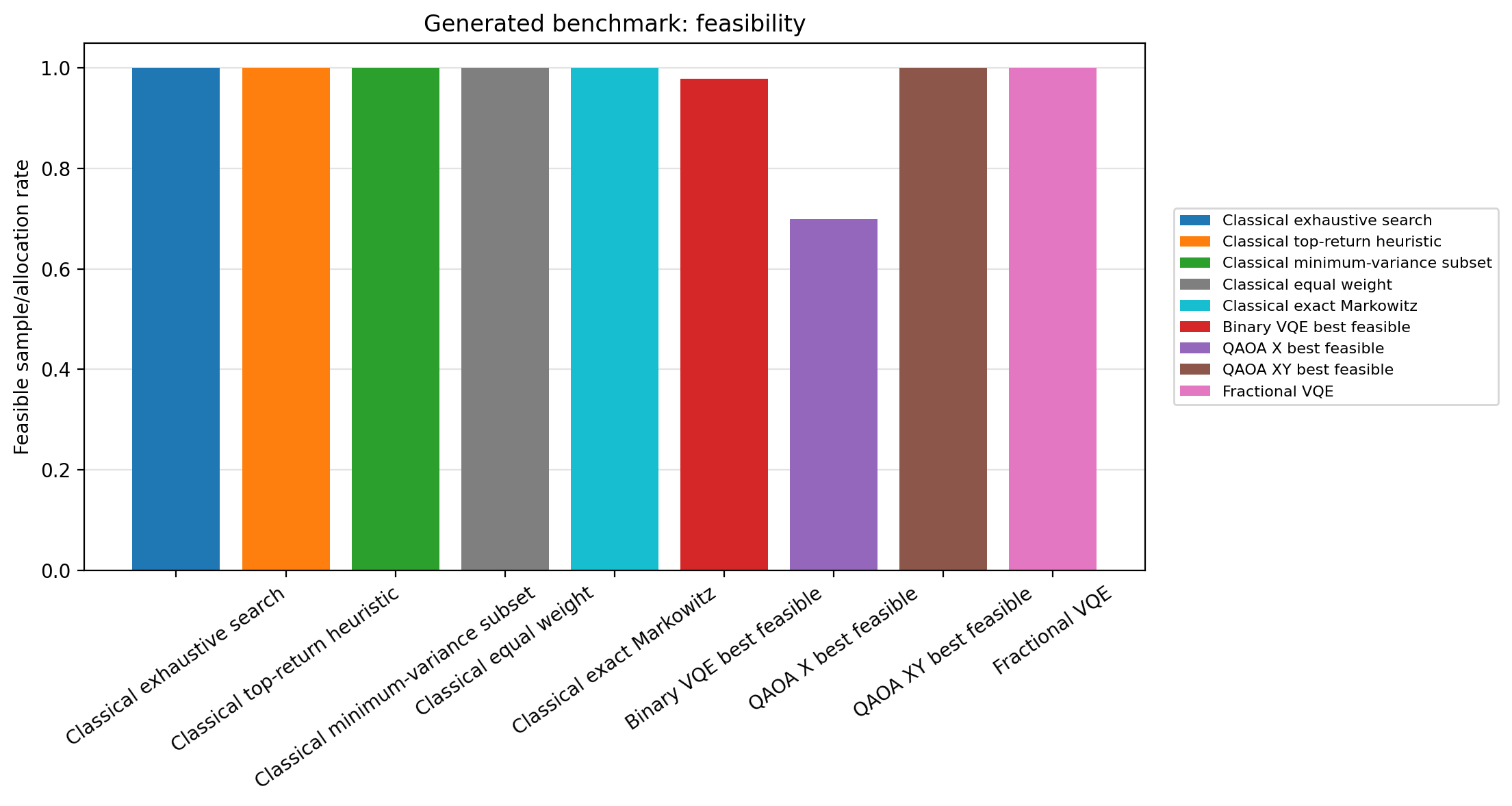
By default this writes results/generated_comparison_summary.csv with classical baselines, multi-seed quantum summaries, feasibility rates, objectives, risk/return metrics, and runtimes. It also writes results/generated_repeatability_trials.csv with one row per method/seed trial. Use --asset-counts, --seeds, --steps, and --methods to expand or tighten the run.

How to Read the Tables

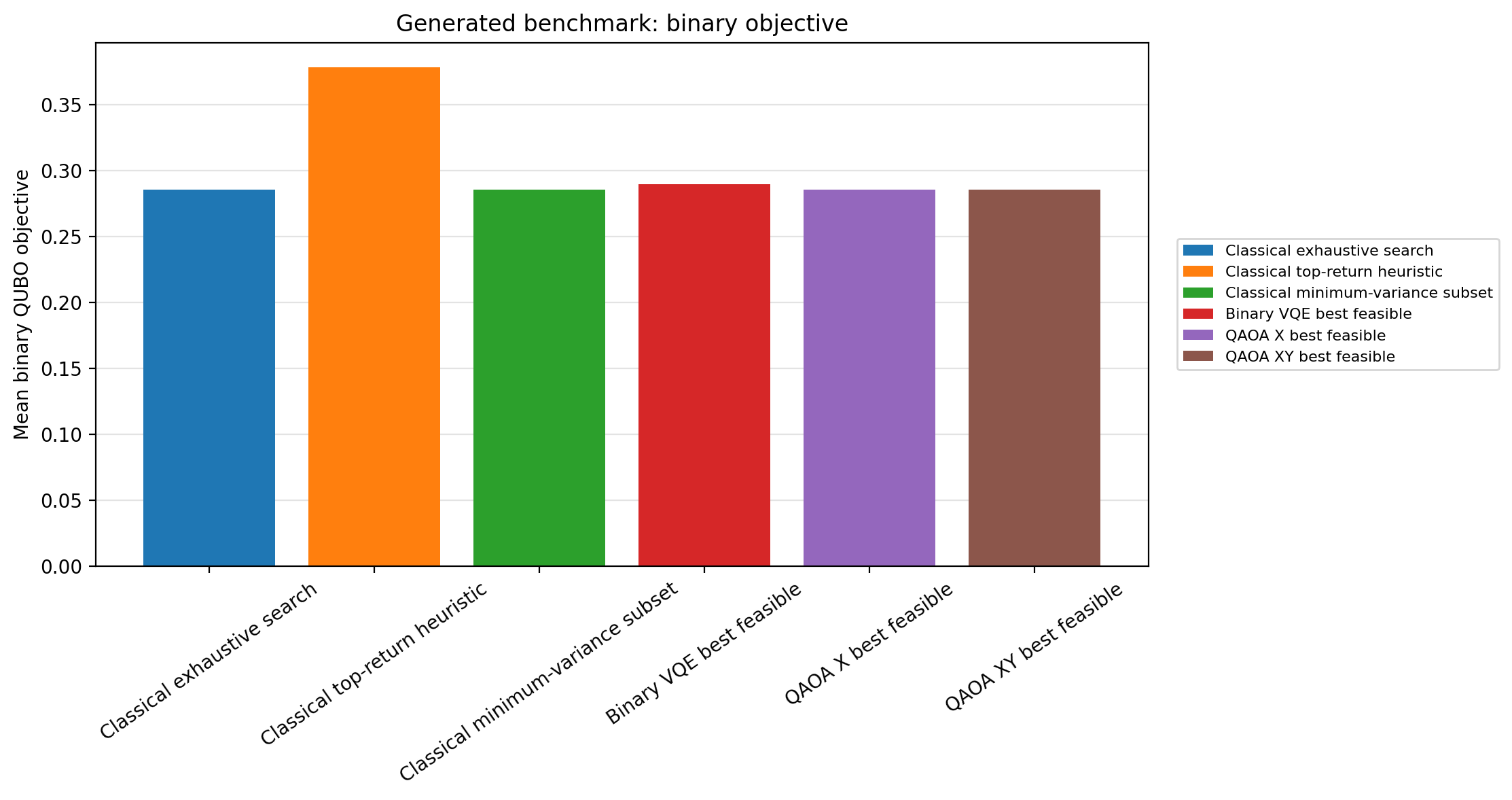
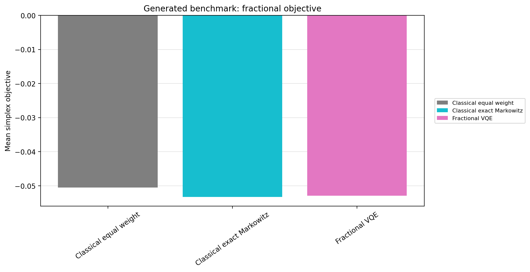
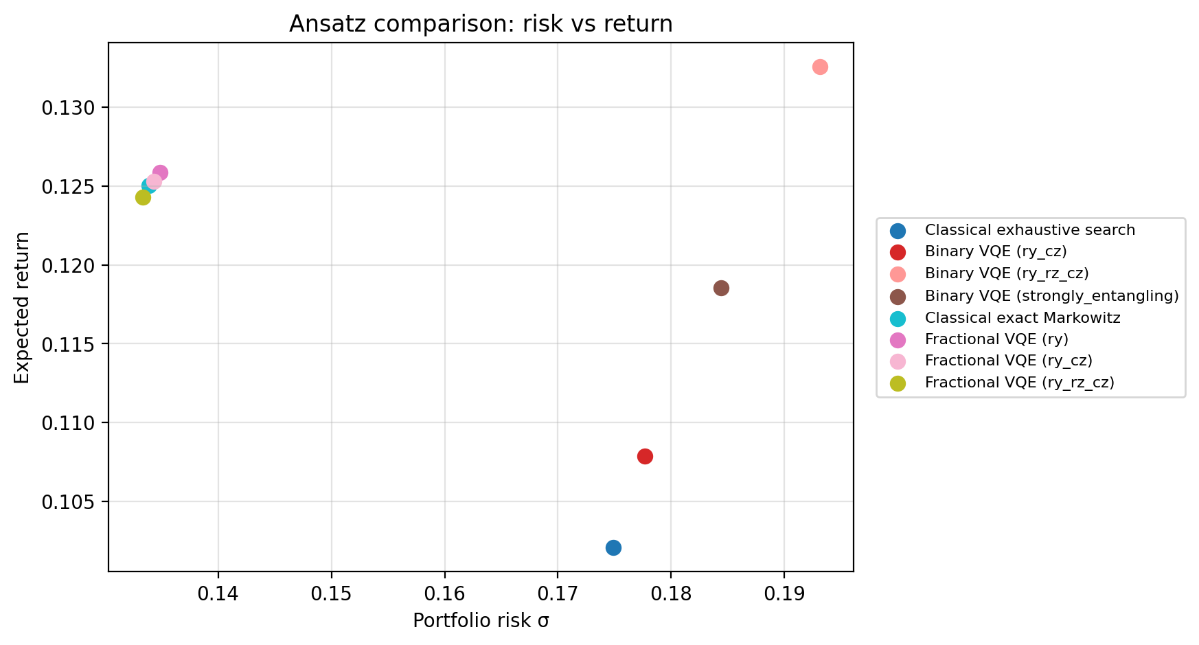
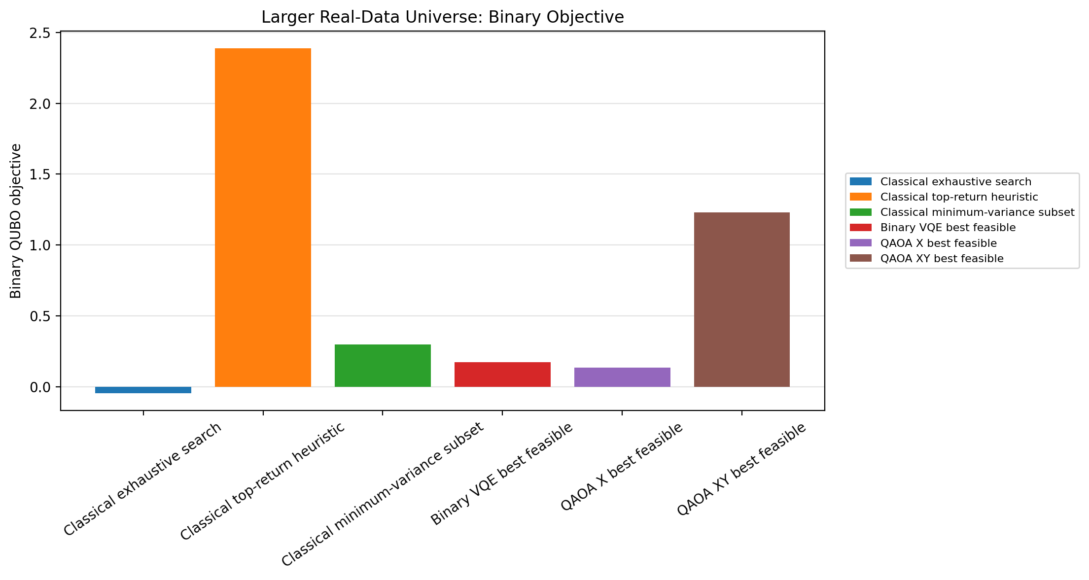
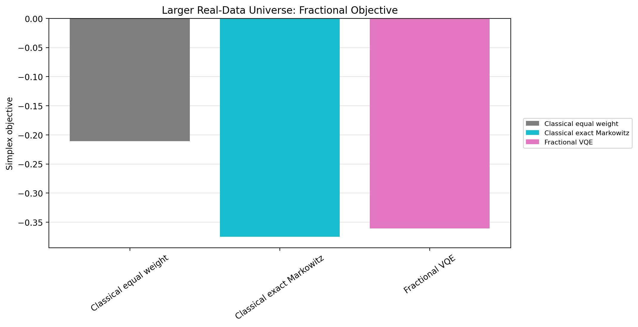
For binary selection methods, lower objective is better for a fixed dataset, risk-aversion value, penalty, and cardinality. For fractional allocation methods, lower simplex objective is better at the same risk-aversion value.

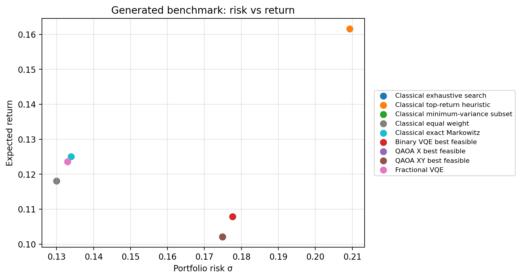
Generated comparison tables include objective_family and reported_weighting columns because binary QUBO objectives and fractional simplex objectives are different mathematical objectives. In generated comparison rows, binary return and risk are reported from equal-weight selected portfolios (x / K) so risk-return plots are comparable with simplex allocations, while the binary objective remains the true QUBO objective evaluated on the raw bitstring x.

The real-data tables report values already saved in notebook outputs. Exact real-data classical optimizer rows should be regenerated together with the market-data notebooks because adjusted prices and shrinkage estimates are provider-dependent.

Synthetic Results

Synthetic examples use fixed in-notebook arrays and are therefore the best place for deterministic method-to-baseline comparisons.

Generated Baseline and Repeatability Results

The generated comparison files add baseline rows and repeatability summaries from deterministic synthetic data:

• Binary baselines: exact exhaustive search, top-return subset, and minimum-variance subset

• Continuous baselines: equal-weight allocation and exact long-only Markowitz

• Quantum repeatability: Binary VQE, QAOA X, QAOA XY, and Fractional VQE summarized across seeds, with per-seed rows saved separately

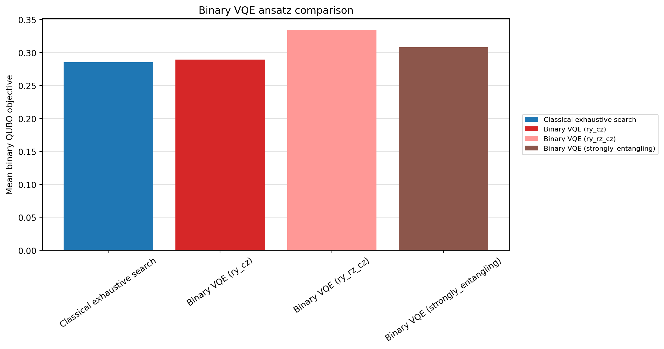
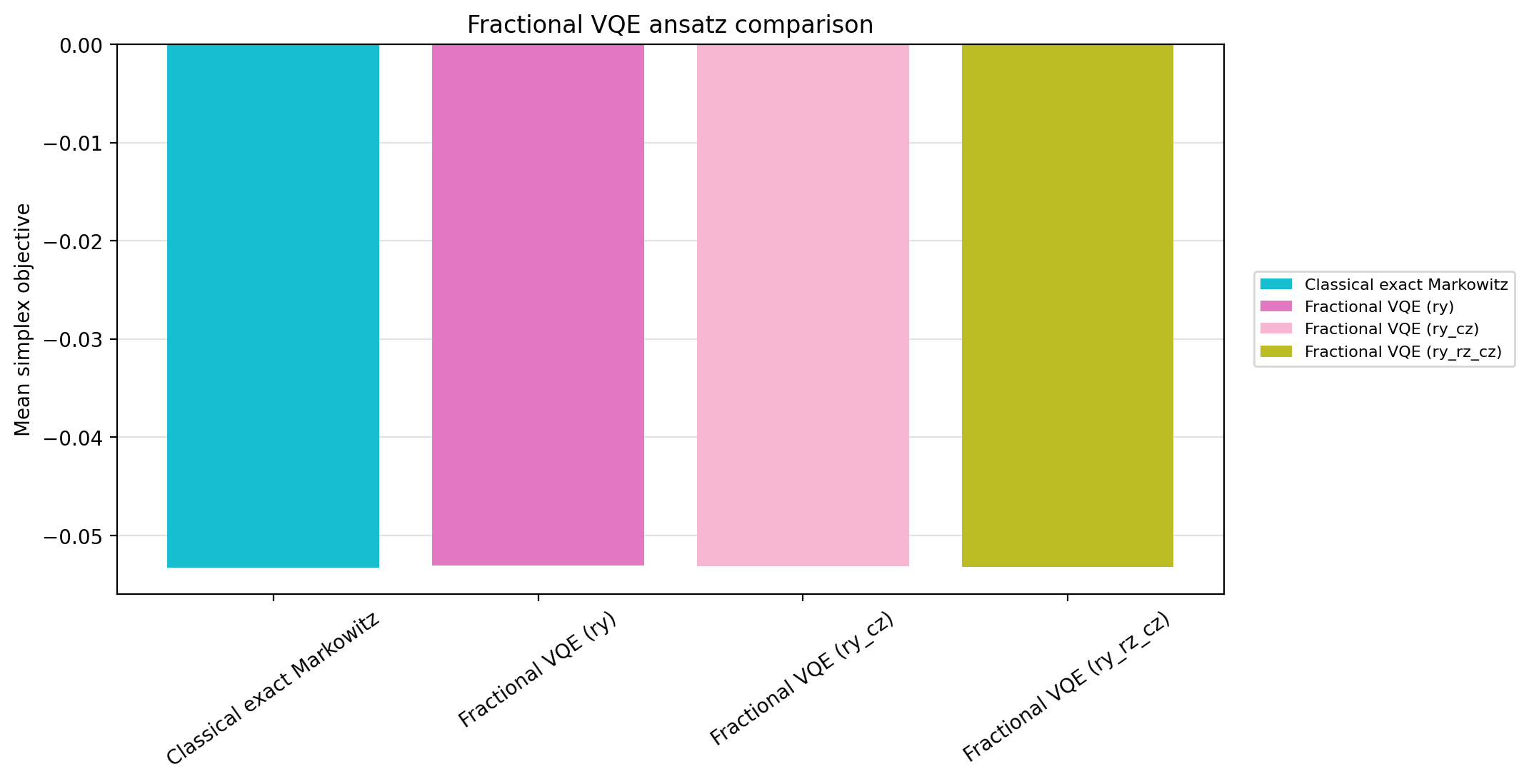
• Objective plots are split by objective family so binary QUBO objectives are not visually mixed with fractional simplex objectives

The committed generated CSVs are lightweight benchmark artifacts. Regenerate them after algorithm changes with:

python scripts/generate_comparison_results.py

Dataset	Method	Objective family	Reported weighting	Seeds	Mean return	Mean risk	Best objective	Mean objective	Std objective	Feasible rate
Synthetic generated n=4	Classical exhaustive search	binary QUBO	equal-weight selected	1	0.102055	0.174865	0.285137	0.285137	0.000000	1.000000
Synthetic generated n=4	Classical top-return heuristic	binary QUBO	equal-weight selected	1	0.161566	0.209324	0.377932	0.377932	0.000000	1.000000
Synthetic generated n=4	Classical minimum-variance subset	binary QUBO	equal-weight selected	1	0.102055	0.174865	0.285137	0.285137	0.000000	1.000000
Synthetic generated n=4	Classical equal weight	fractional simplex	simplex weights	1	0.118063	0.129968	-0.050496	-0.050496	0.000000	1.000000
Synthetic generated n=4	Classical exact Markowitz	fractional simplex	simplex weights	1	0.125046	0.133935	-0.053292	-0.053292	0.000000	1.000000
Synthetic generated n=4	Binary VQE best feasible	binary QUBO	equal-weight selected	3	0.107872	0.177643	0.285137	0.289414	0.006049	0.978516
Synthetic generated n=4	QAOA X best feasible	binary QUBO	equal-weight selected	3	0.102055	0.174865	0.285137	0.285137	0.000000	0.699219
Synthetic generated n=4	QAOA XY best feasible	binary QUBO	equal-weight selected	3	0.102055	0.174865	0.285137	0.285137	0.000000	1.000000
Synthetic generated n=4	Fractional VQE	fractional simplex	simplex weights	3	0.123596	0.132920	-0.053289	-0.052921	0.000415	1.000000

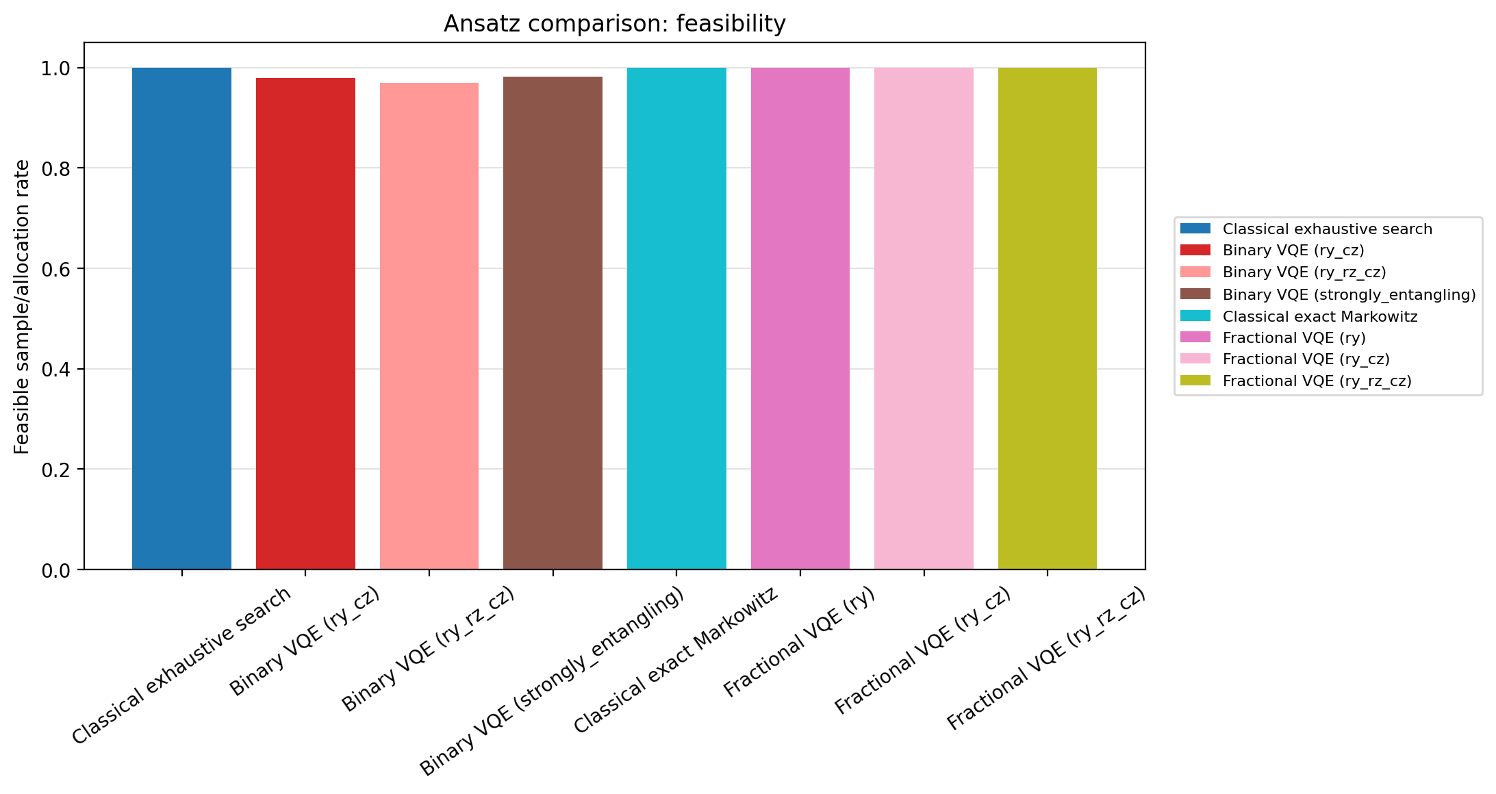
Ansatz Comparison Results

The ansatz comparison notebook is a compact pure-package client for the Binary VQE and Fractional VQE ansatz options. It writes results/ansatz_comparison.csv and keeps method/ansatz colors consistent across its risk-return, objective, and feasibility plots.

Regenerate it with:

python scripts/generate_ansatz_comparison.py

Synthetic Discrete Selection

Dataset	Method	Type	λ	K	Selection	Return	Risk	Variance	Objective	Feasible
Synthetic binary toy	Classical exhaustive search	Classical	5.0	2	1100	0.300000	0.158114	0.025000	-0.175000	yes
Synthetic binary toy	Binary VQE Top-K	Quantum	5.0	2	0101	0.320000	0.256905	0.066000	0.010000	yes
Synthetic QAOA toy	Classical exhaustive search	Classical	4.0	2	1001	0.250000	0.360555	0.130000	0.270000	yes
Synthetic QAOA toy	QAOA X/XY best feasible	Quantum	4.0	2	1001	0.250000	0.360555	0.130000	0.270000	yes
Synthetic QAOA toy	QAOA X/XY Top-K	Quantum	4.0	2	0011	0.220000	0.387298	0.150000	0.380000	yes

Synthetic Continuous Allocation

Dataset	Method	Type	λ	Selection or weights	Return	Risk	Objective	Feasible
Synthetic fractional toy	Classical Markowitz	Classical	5.0	[0.480403, 0.355580, 0.131539, 0.032477]	0.142785	0.059812	-0.124897	yes
Synthetic fractional toy	Fractional VQE	Quantum	5.0	continuous allocation	0.142792	0.059825	not printed	simplex-normalized

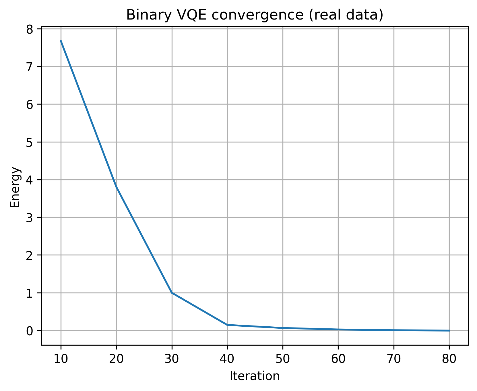
Binary VQE Synthetic Figures

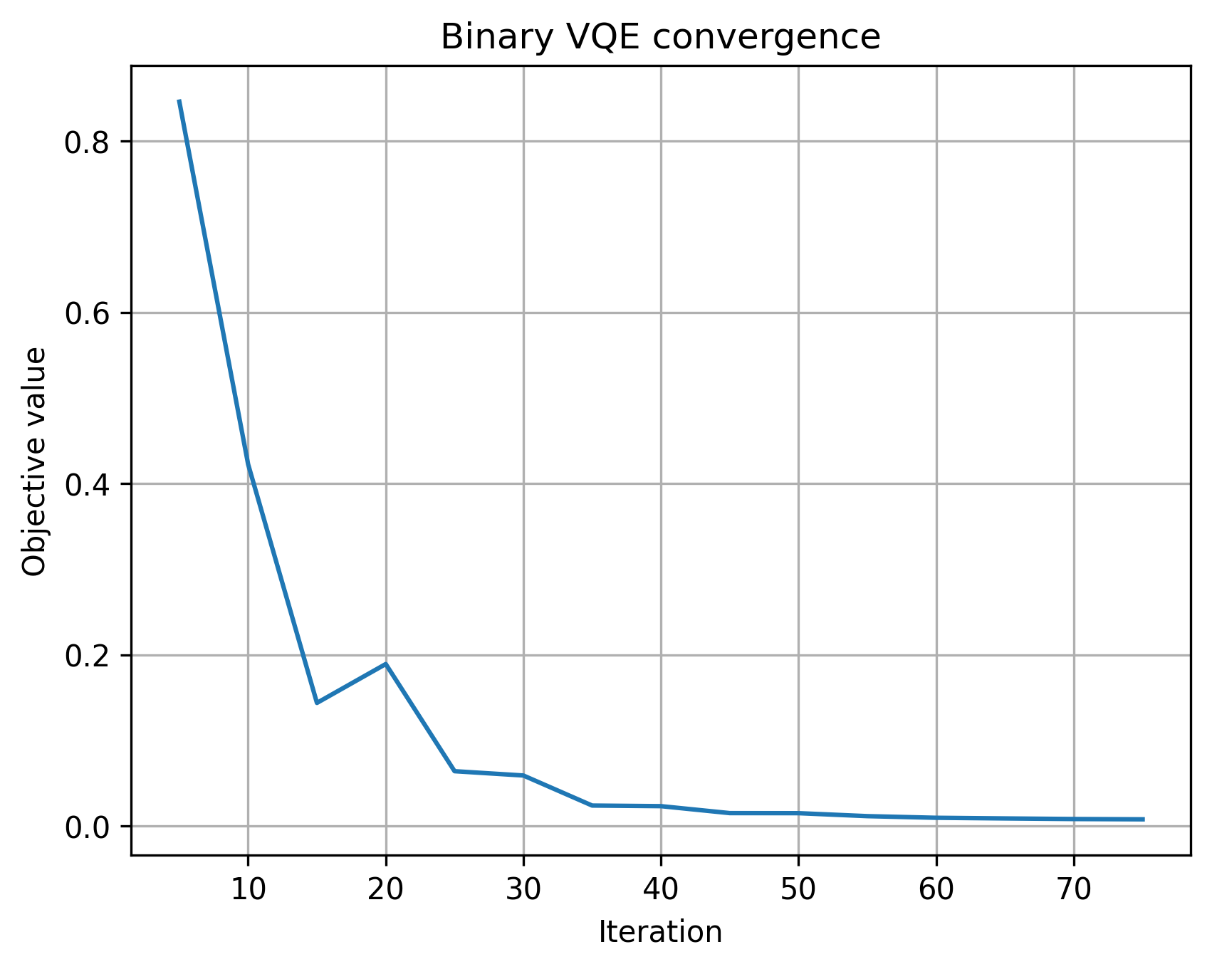
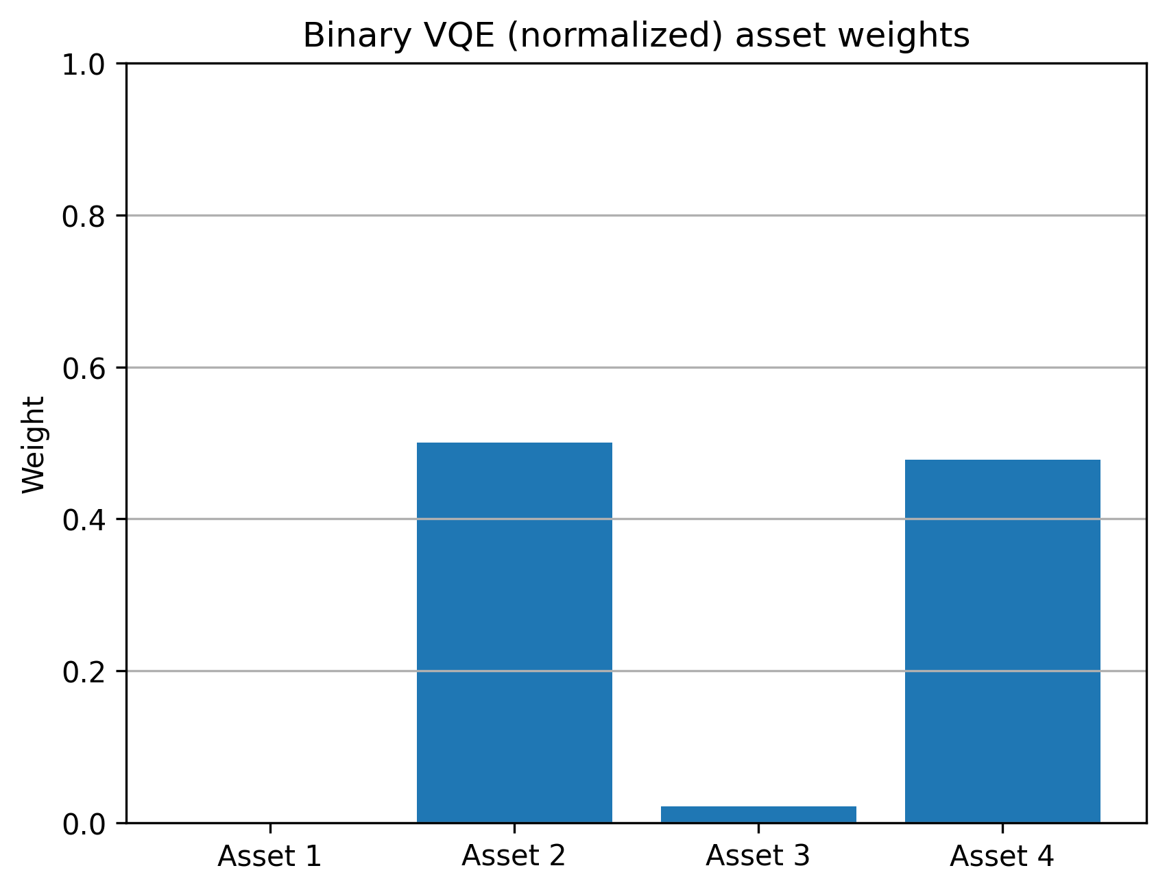
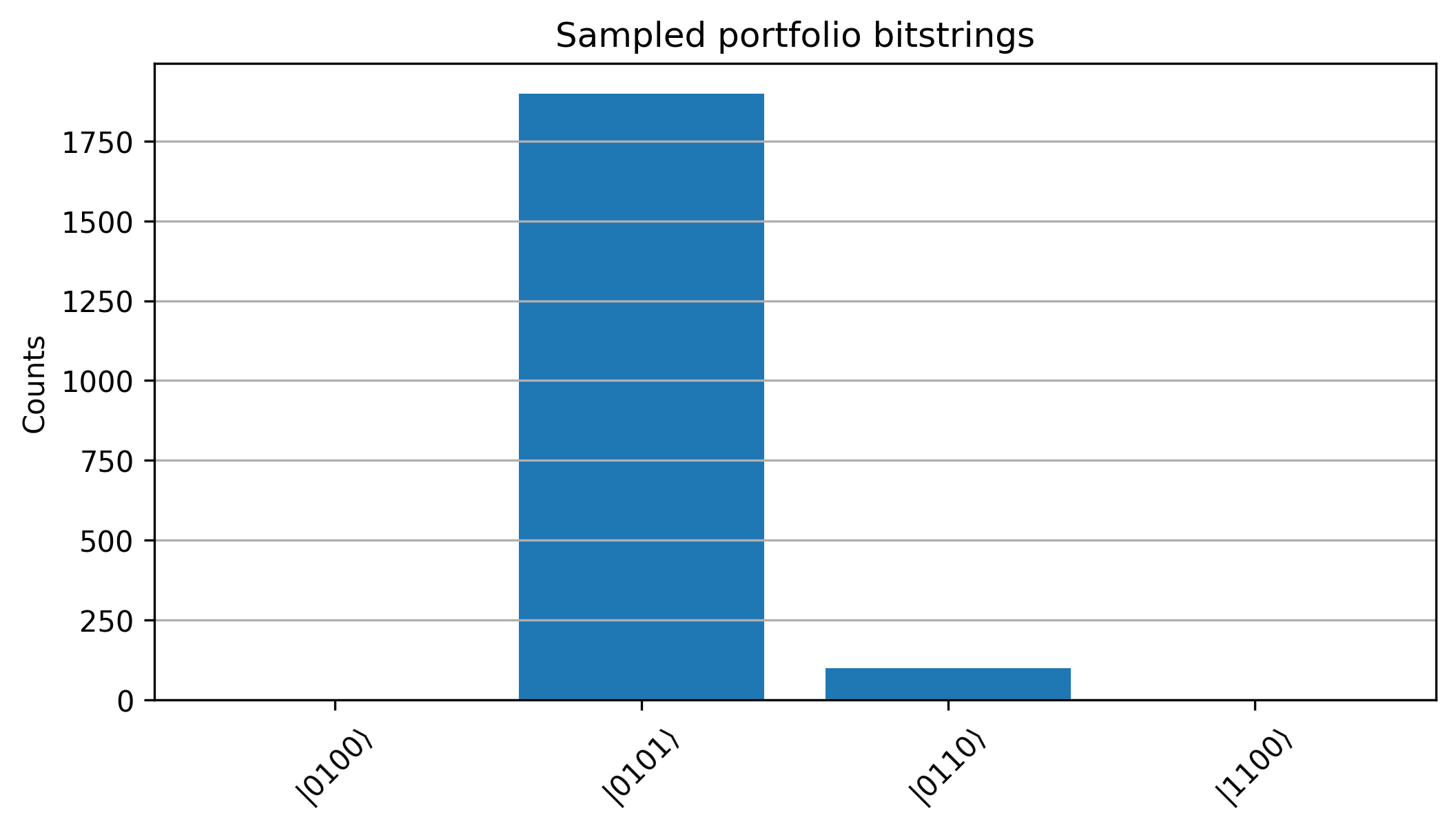
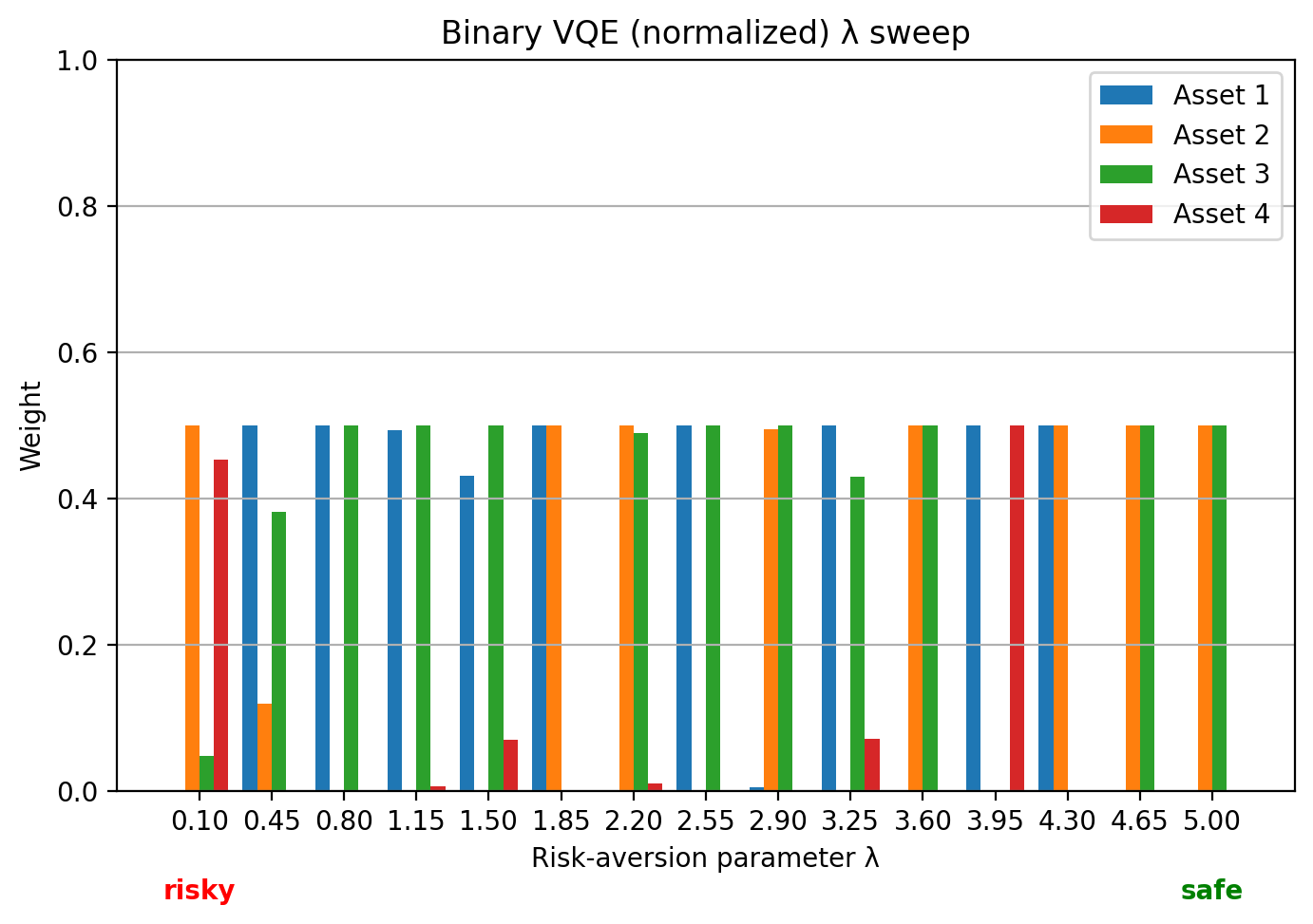
Binary VQE solves a cardinality-constrained portfolio selection problem by mapping the QUBO objective to an Ising Hamiltonian and minimizing its expectation value with a parameterized circuit.

Artifact	What it shows
Circuit	Hardware-efficient binary VQE ansatz used by the notebook client
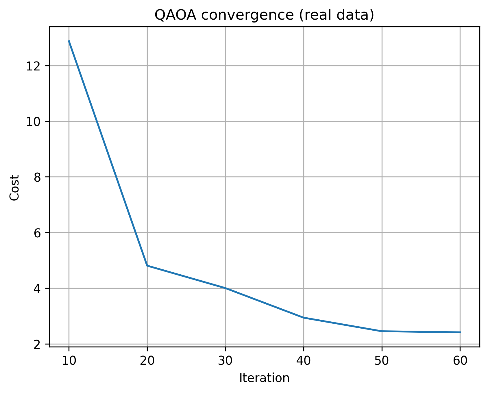
Convergence	Optimizer cost trace over training steps
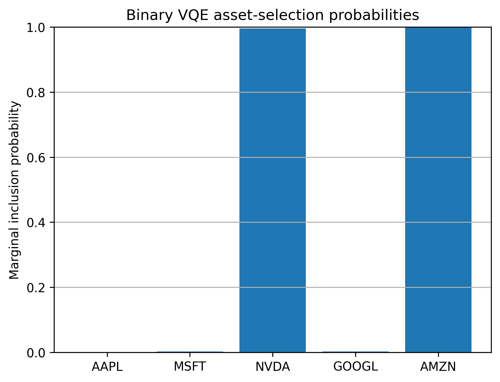
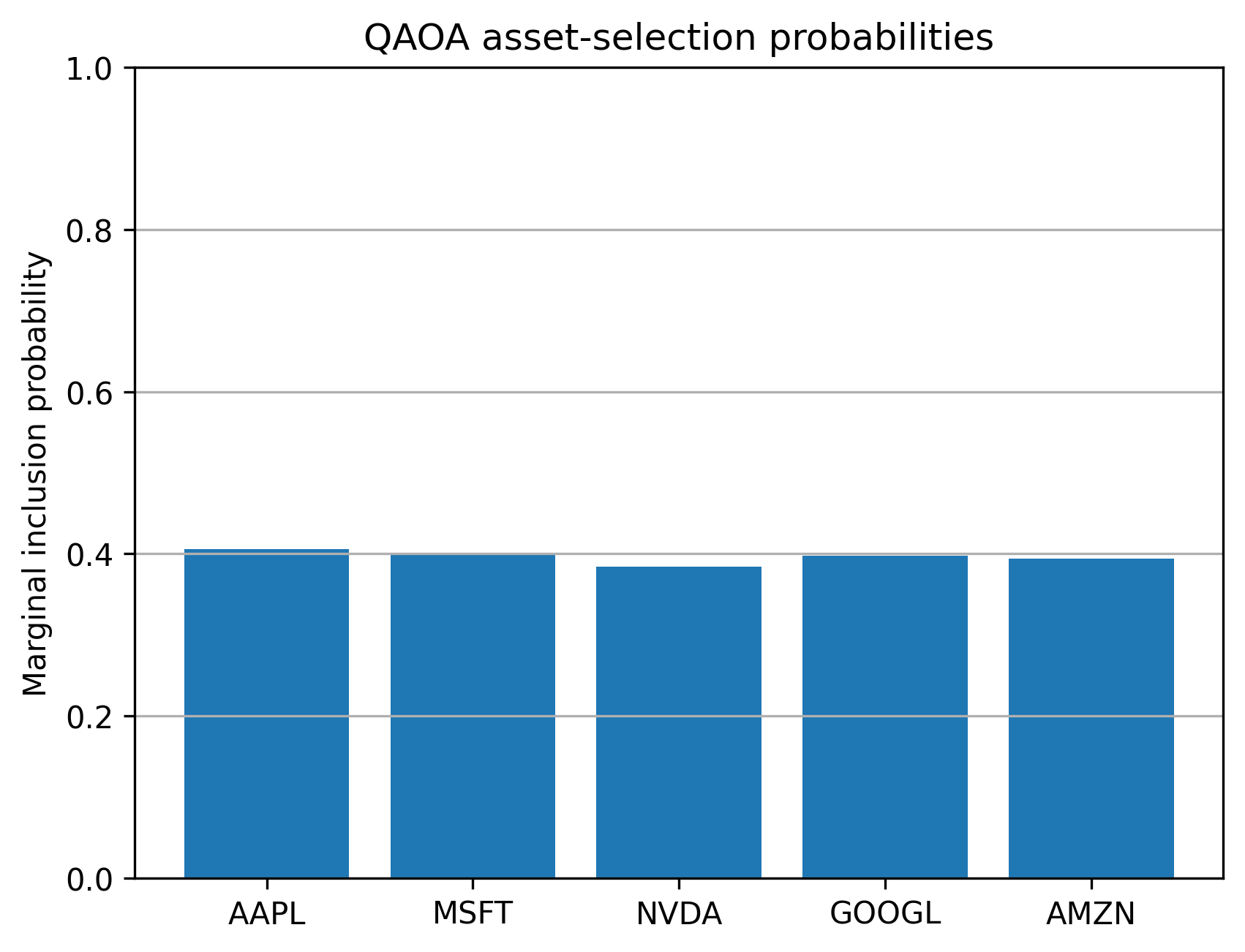
Probabilities	Selection probability distribution after optimization
Bitstrings	Most likely sampled portfolio bitstrings
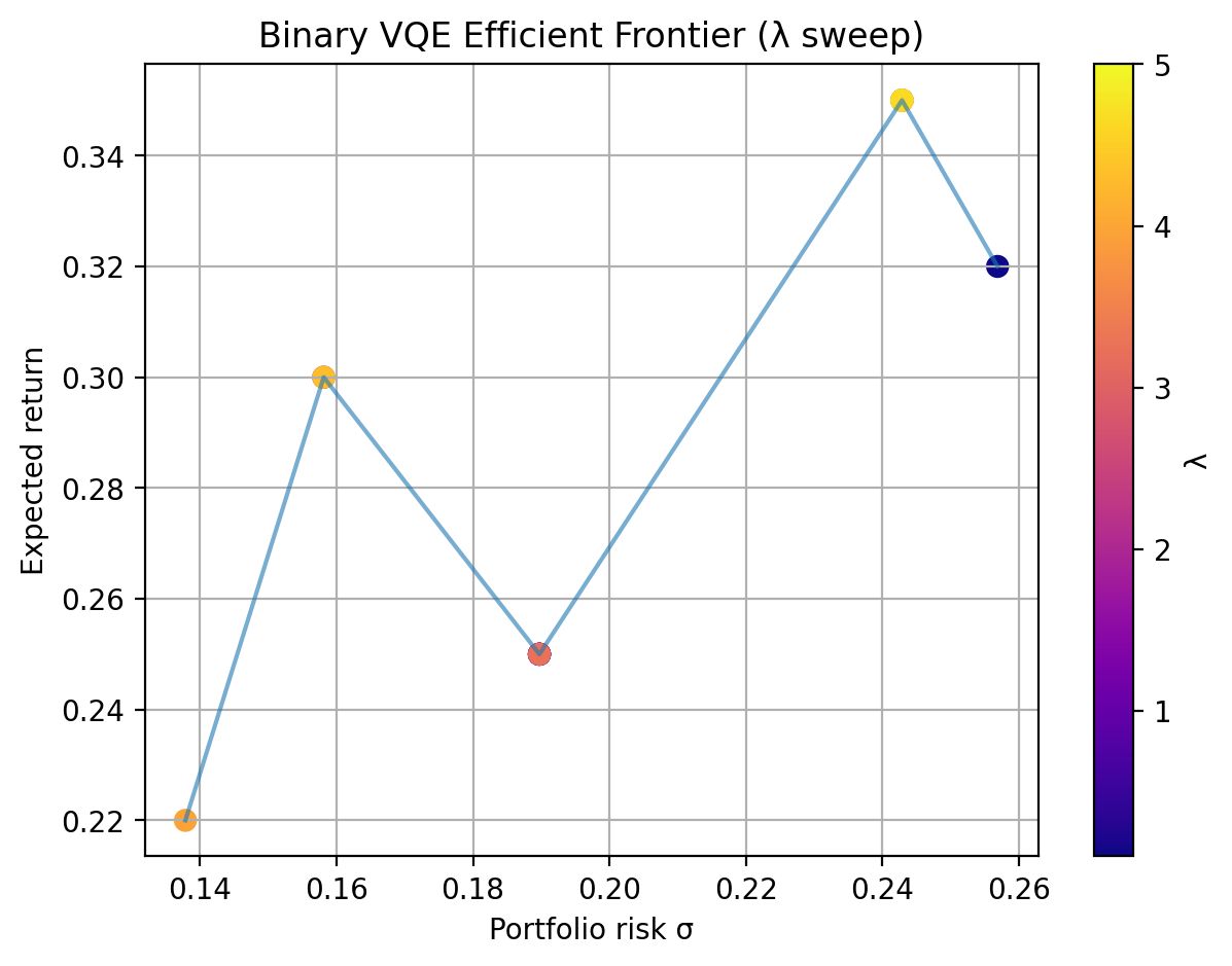
Lambda sweep	Risk-return behavior as the risk-aversion parameter changes
Efficient frontier	Binary candidates compared across return/risk tradeoffs

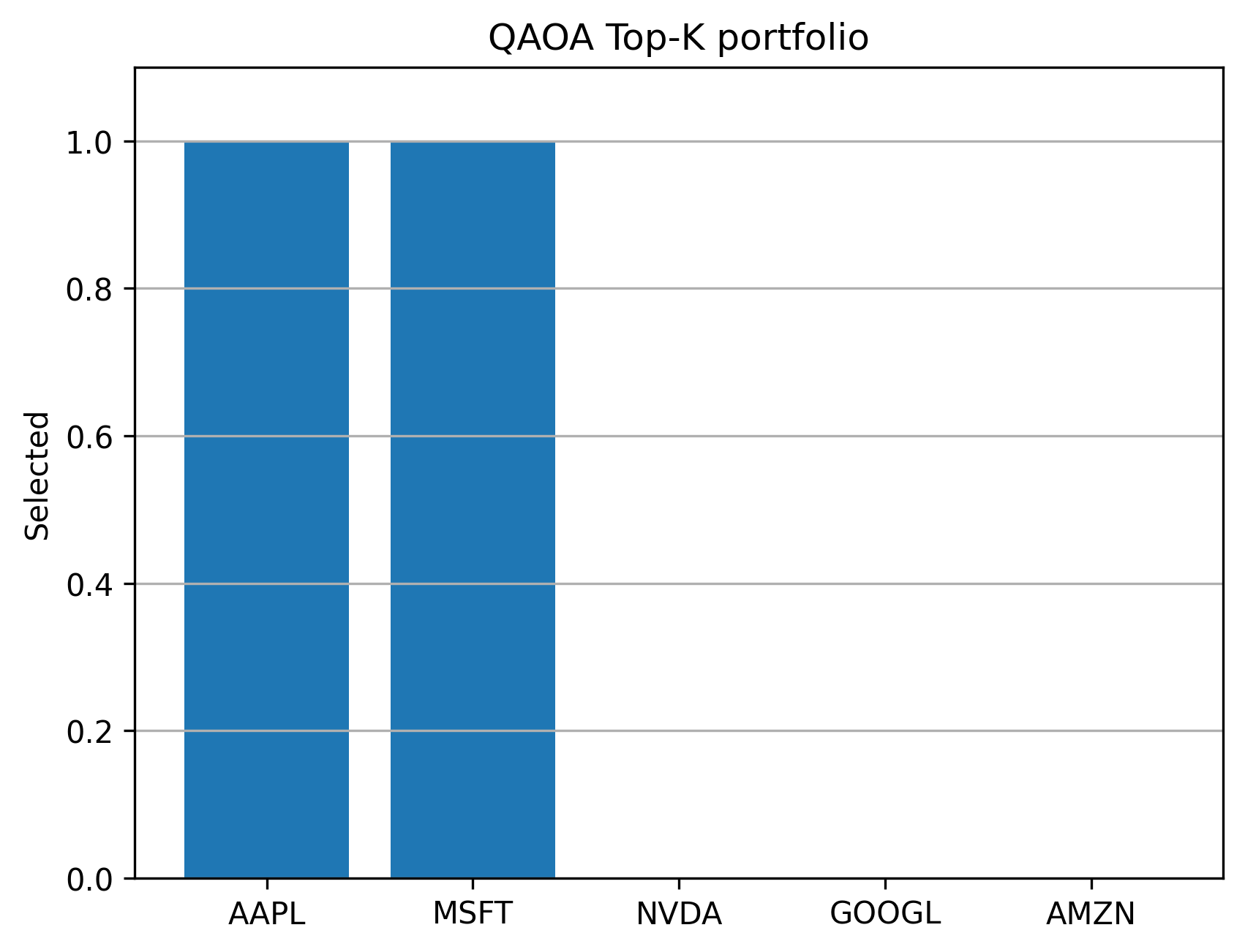
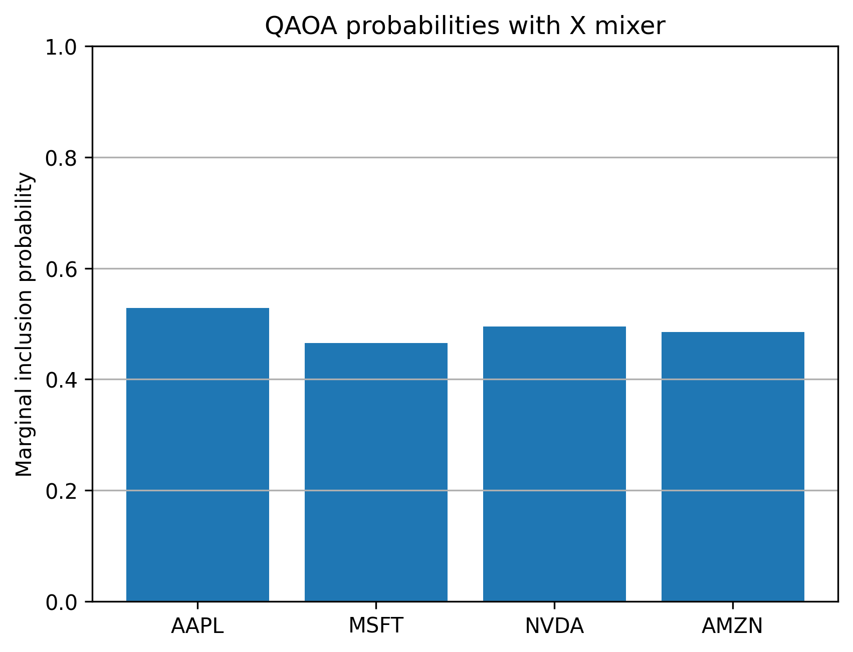
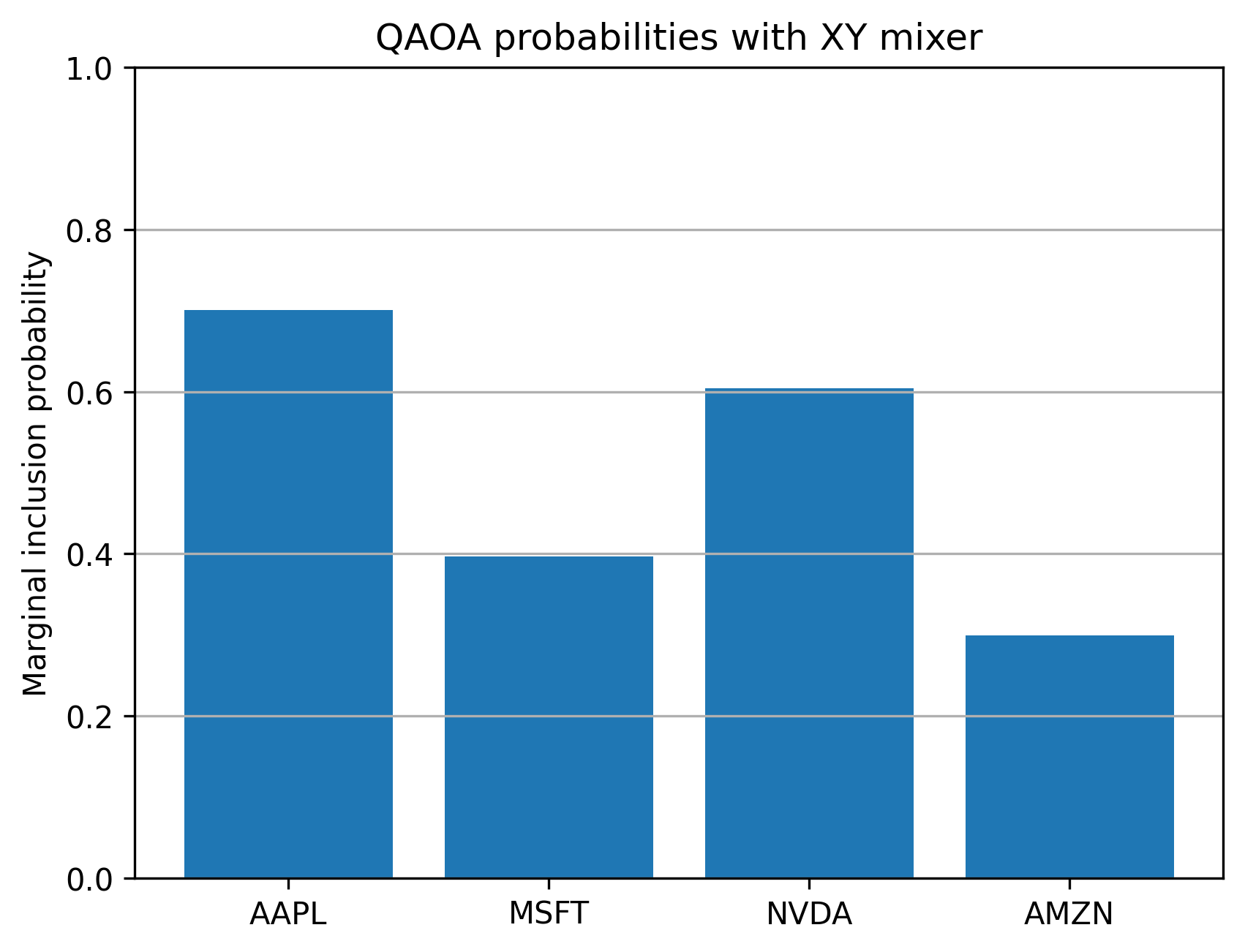
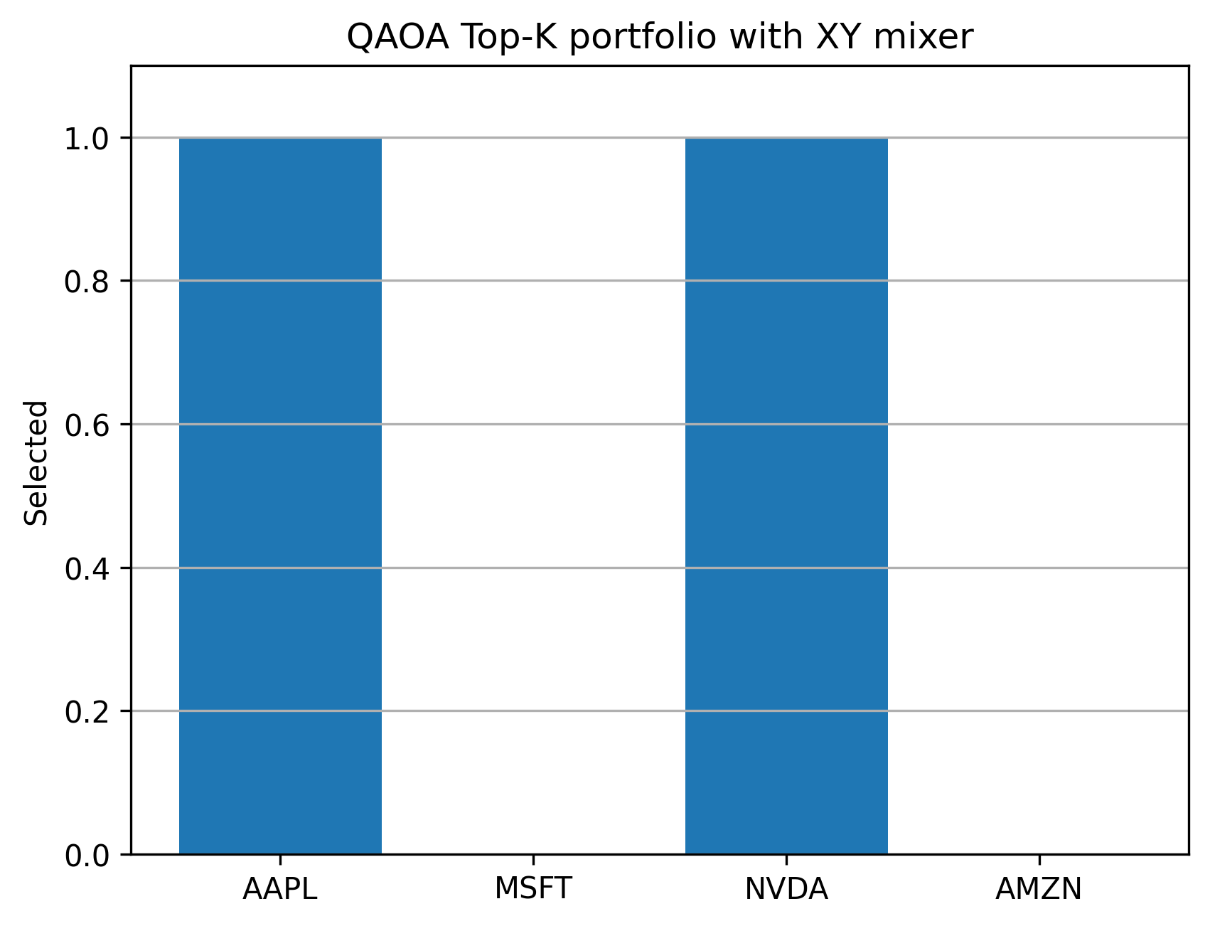
QAOA Synthetic Figures

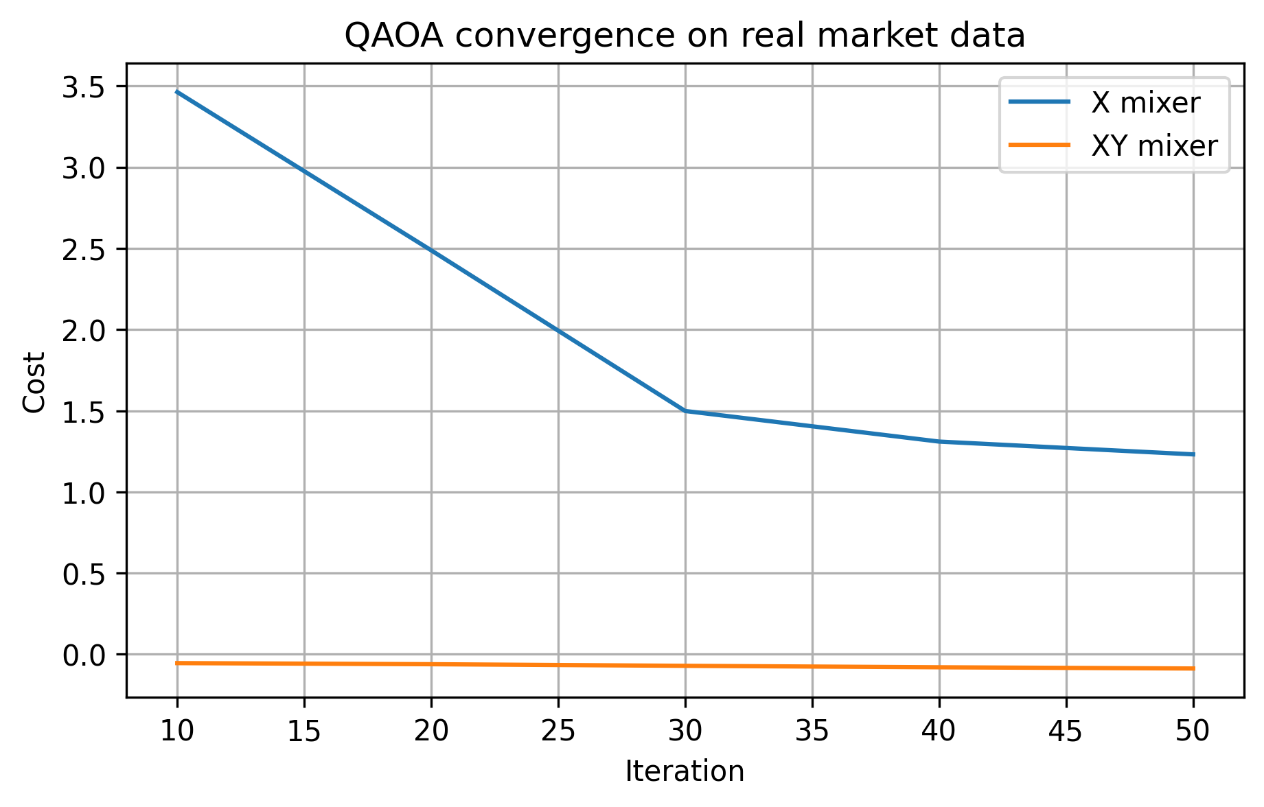
QAOA solves the binary portfolio objective with alternating cost and mixer unitaries. The synthetic notebook compares standard X-mixer sampling with constraint-aware XY-mixer behavior.

Artifact	What it shows
Candidate comparison	Top-K, mode, and best-feasible sampled bitstrings
Mixer comparison	X and XY mixer behavior on the same binary objective
Final portfolio metrics	Return, quadratic risk, and objective for the selected feasible bitstring

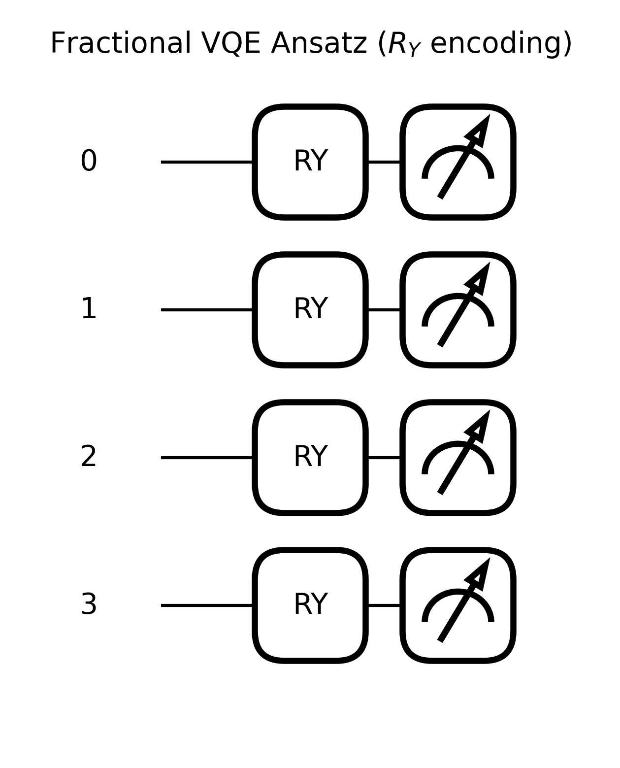
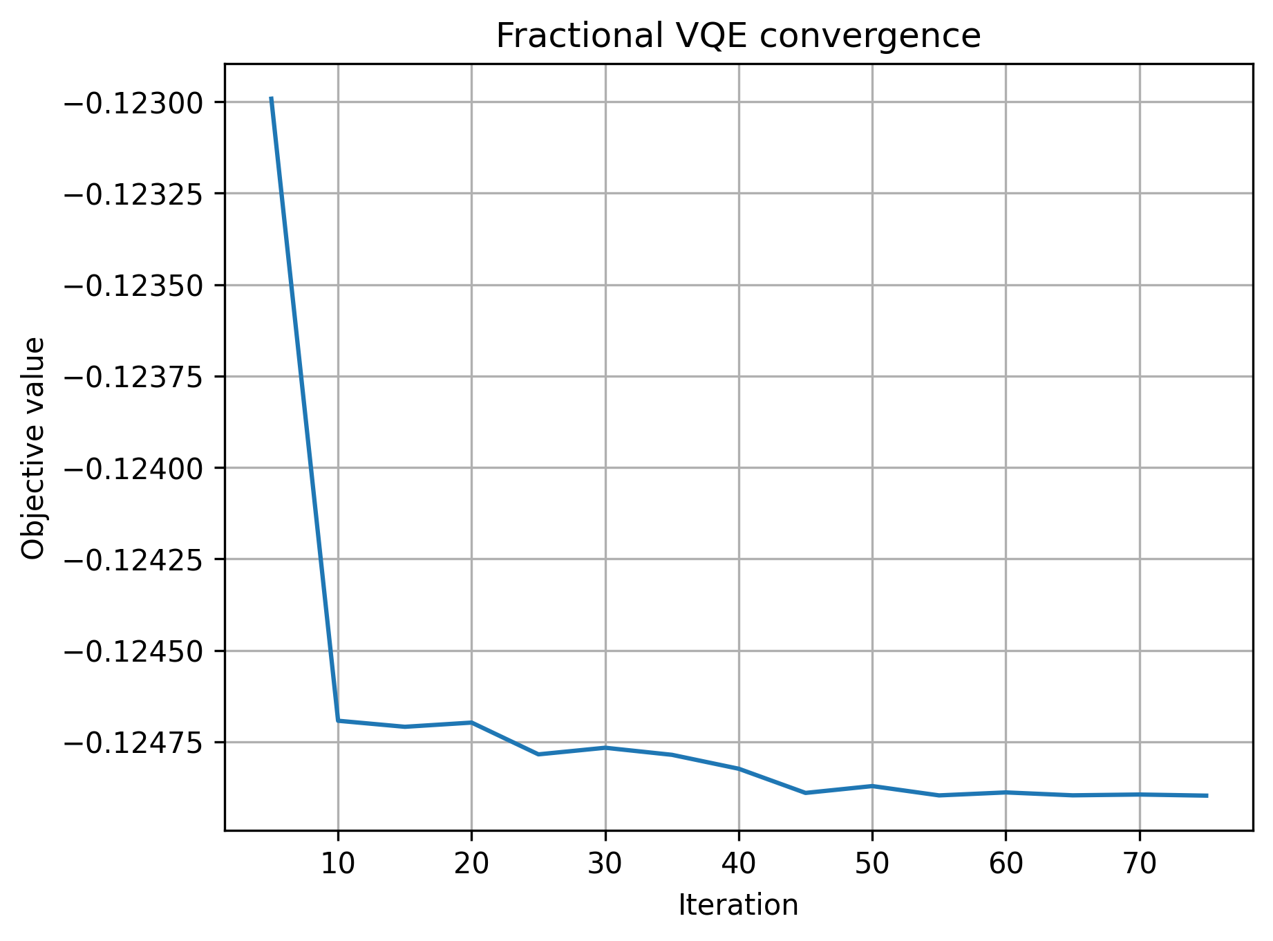
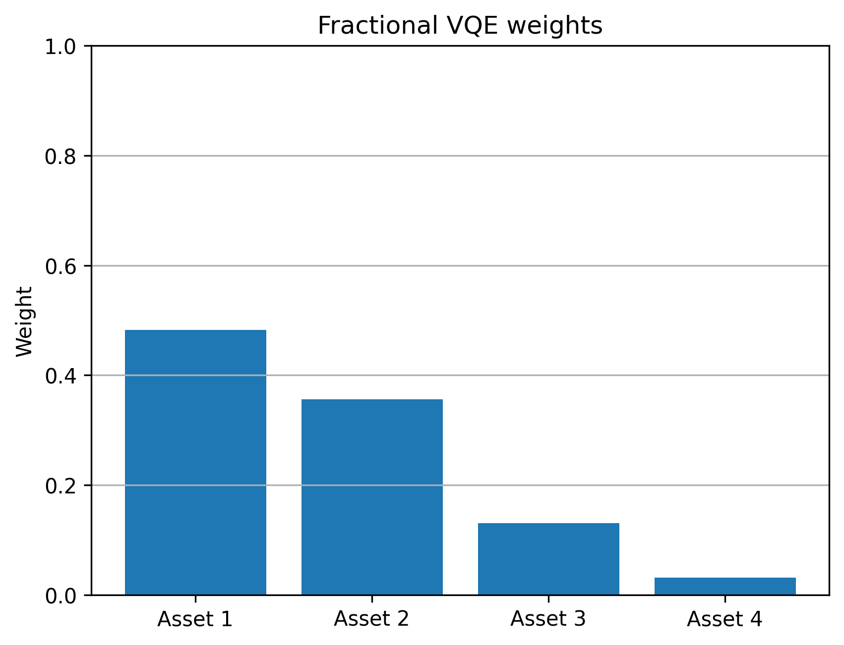
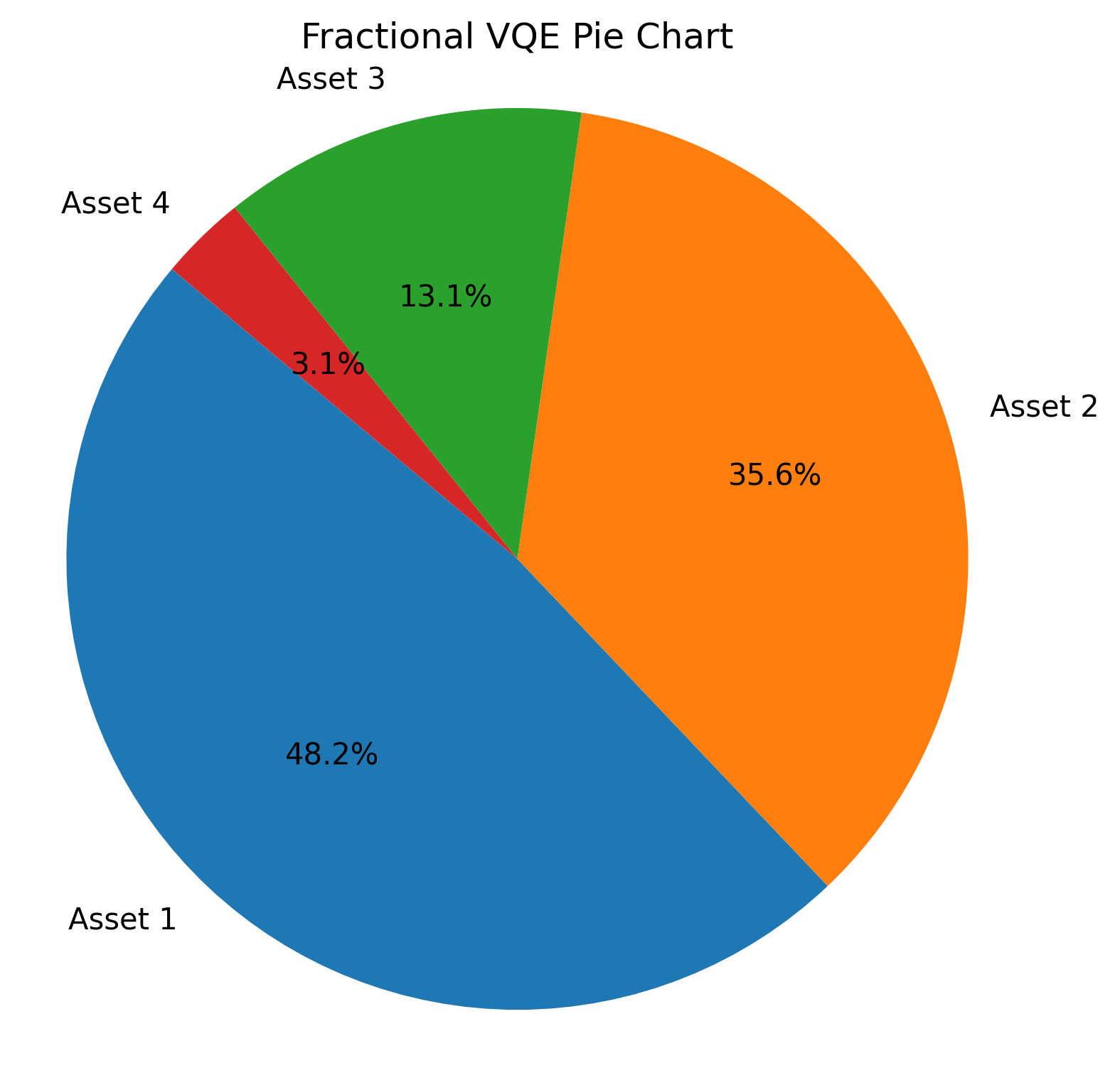
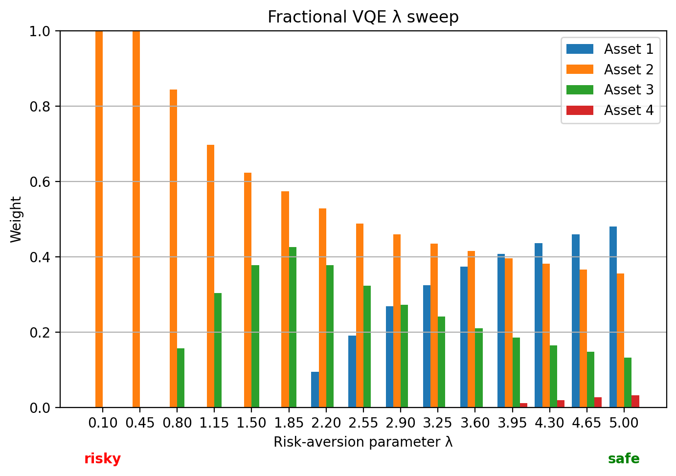
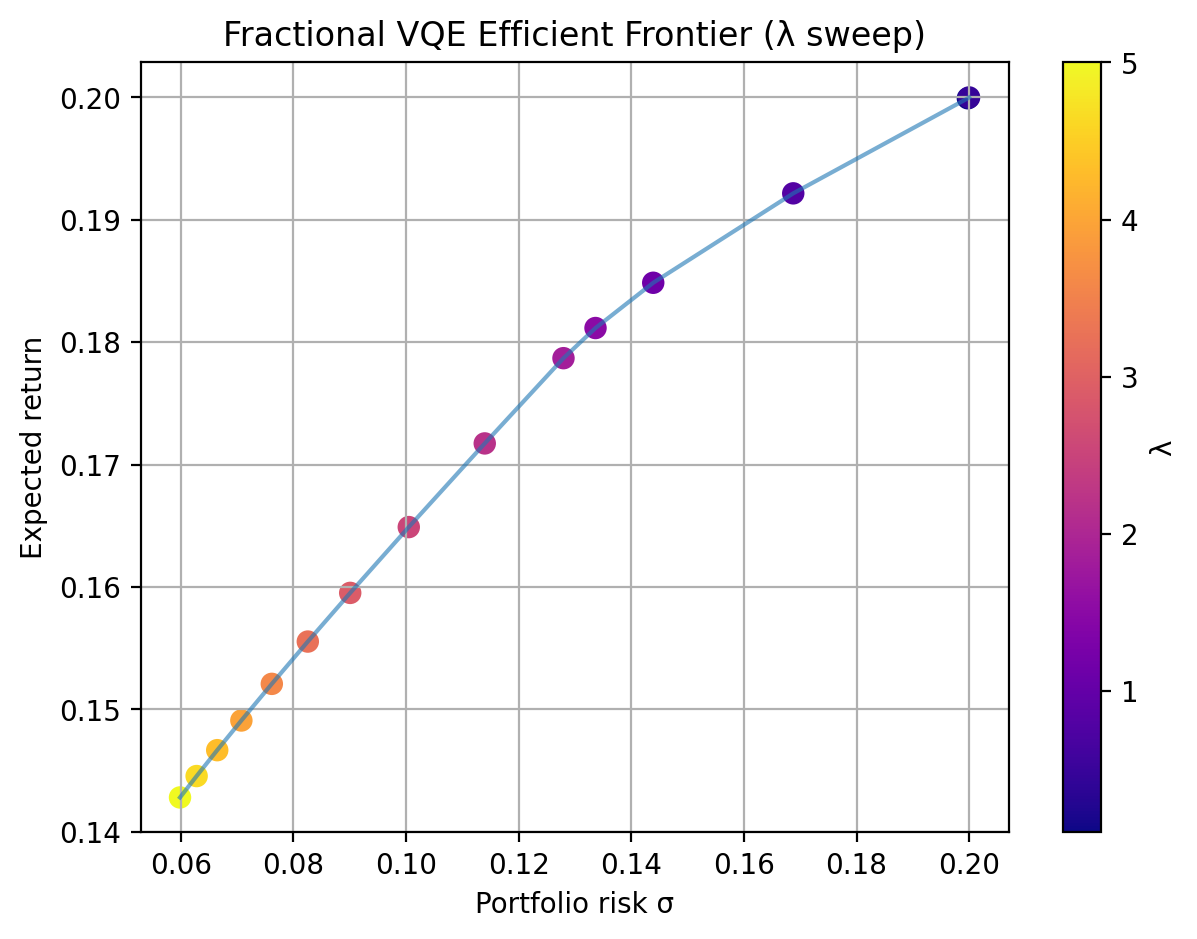
Fractional VQE Synthetic Figures

Fractional VQE optimizes long-only continuous allocations on the simplex. This complements binary selection by producing allocation weights directly rather than choosing a fixed-size subset.

Artifact	What it shows
Circuit	Fractional VQE ansatz used for continuous allocation
Convergence	Optimizer behavior for the fractional objective
Probabilities	Allocation-related distribution from the fractional workflow
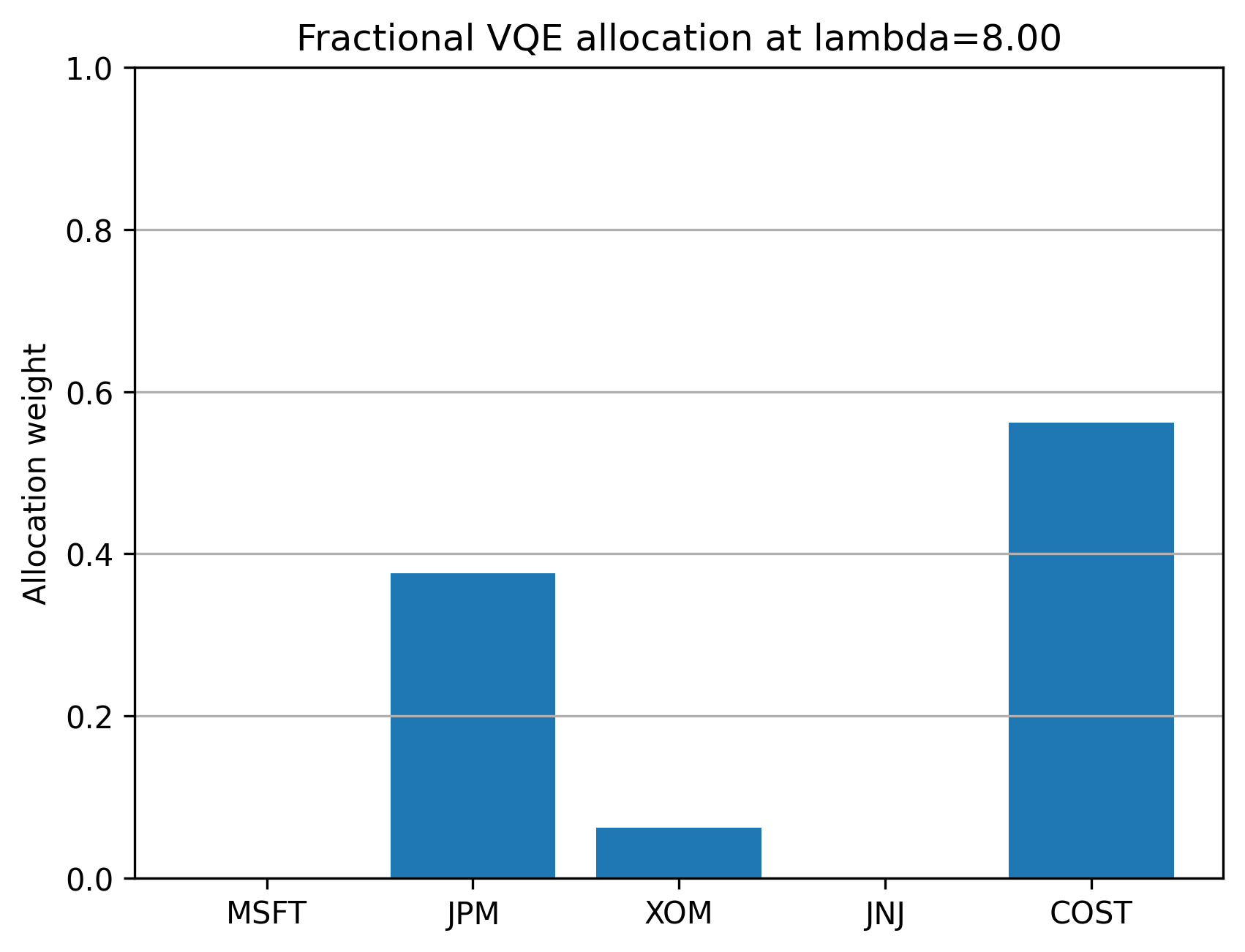
Final allocation	Portfolio weights displayed as a pie chart
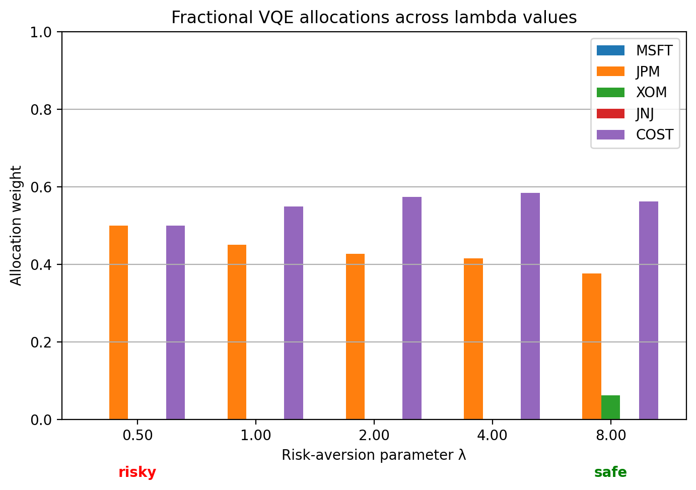
Lambda sweep	Allocation changes over risk-aversion settings
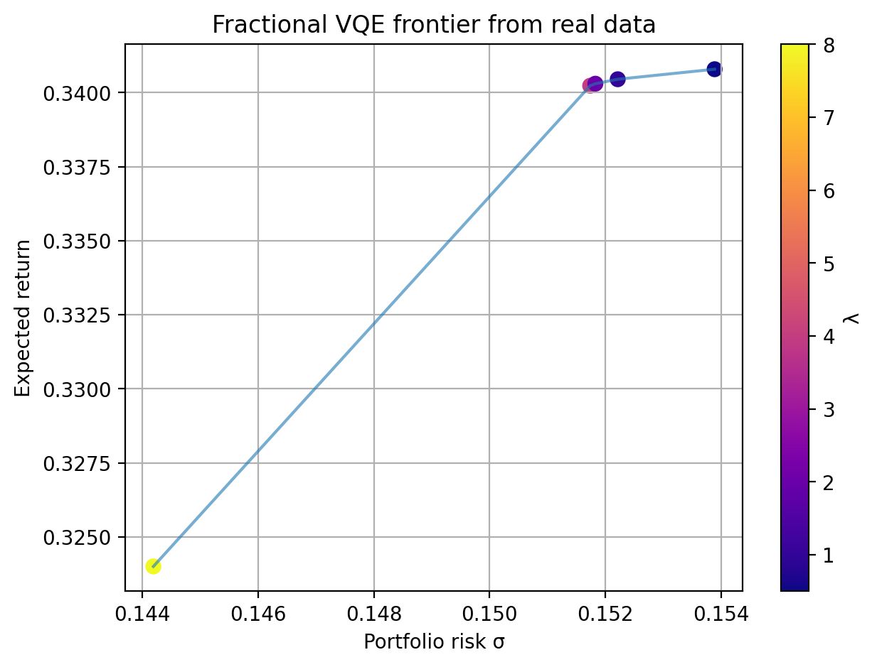
Efficient frontier	Fractional allocation frontier from optimized portfolios

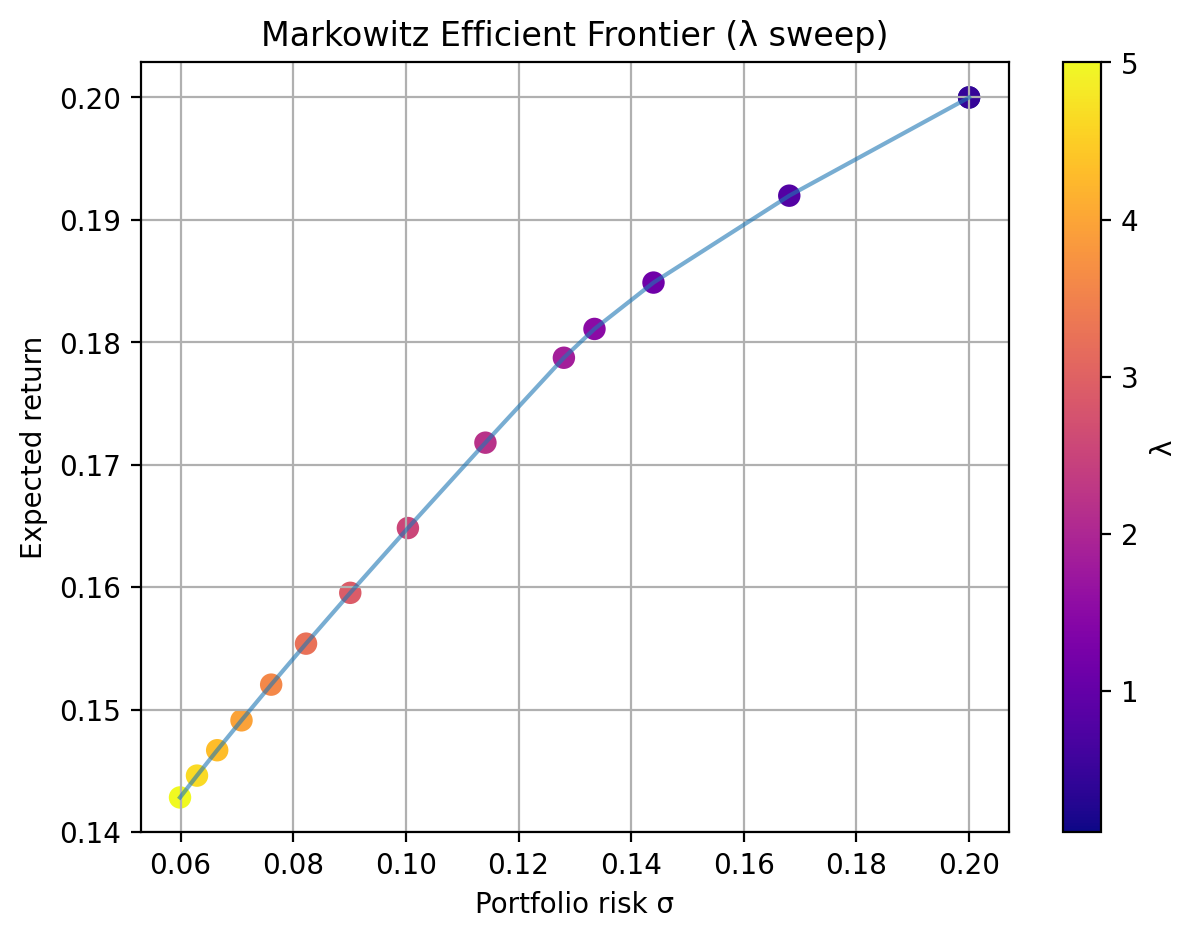
Classical Markowitz Synthetic Figures

The classical Markowitz notebook provides reference plots for interpreting quantum portfolio outputs. These plots are useful for checking whether quantum-generated candidates sit in sensible risk-return regions.

Artifact	What it shows
Risk-return scatter	Candidate portfolios colored by return/risk behavior
Markowitz lambda sweep	Classical allocation changes across risk-aversion settings

Real-Data Results

Real-data notebooks use market data for a fixed 2024-01-01 to 2025-01-01 window. The committed values below come from notebook output cells and should be regenerated whenever the real-data notebooks are rerun.

Real-Data Summary

Dataset	Method	Type	Window	Selection or frontier	Return	Risk	Objective	Feasible
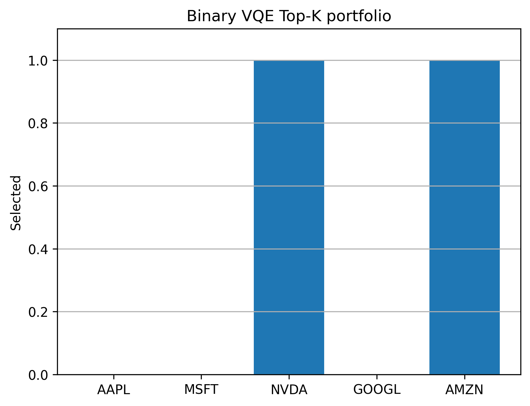
Real binary example	Binary VQE Top-K	Quantum	2024-01-01 to 2025-01-01	NVDA, AMZN	0.681501	0.335301	not printed	yes
Real binary example	Classical equal-weight evaluation	Classical evaluation	2024-01-01 to 2025-01-01	NVDA, AMZN	0.681501	0.335301	not printed	yes
Real QAOA example	QAOA X best feasible	Quantum	2024-01-01 to 2025-01-01	AAPL, NVDA	not printed	not printed	-0.205323	yes
Real QAOA example	QAOA XY best feasible	Quantum	2024-01-01 to 2025-01-01	AAPL, NVDA	not printed	not printed	-0.205323	yes

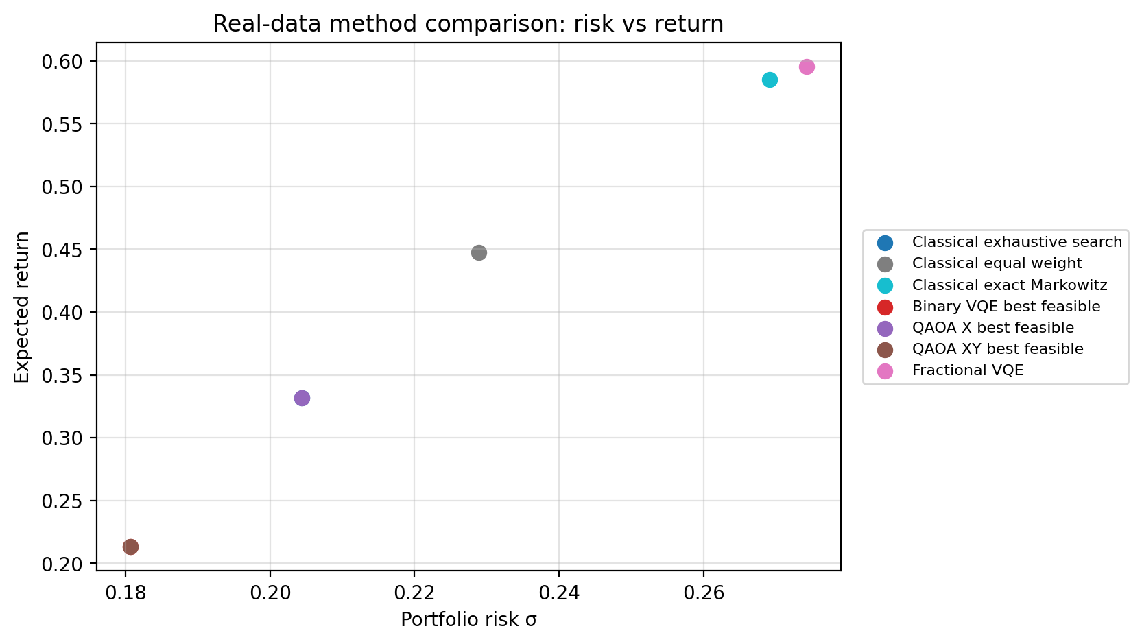
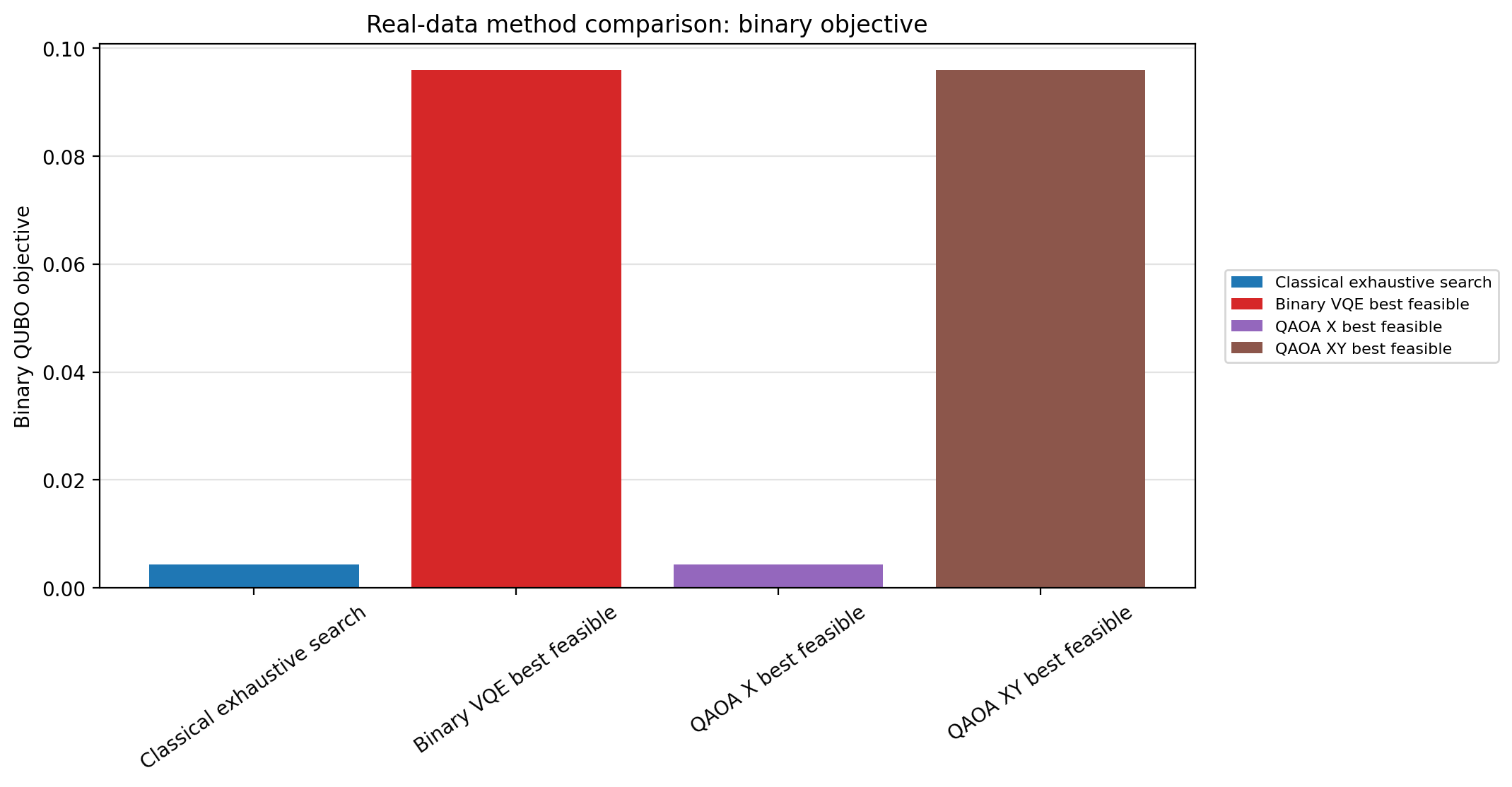
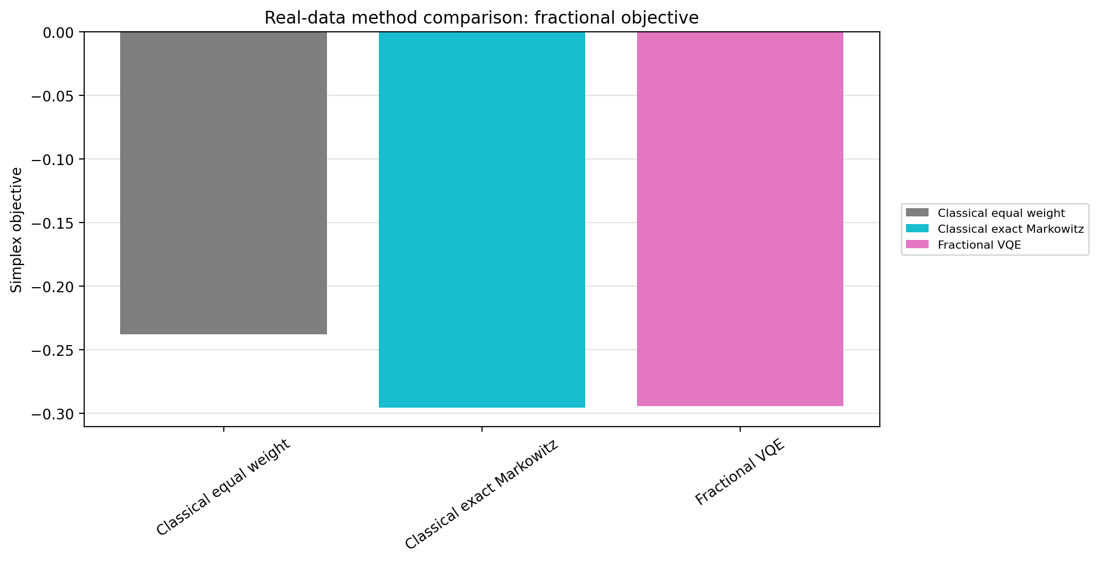
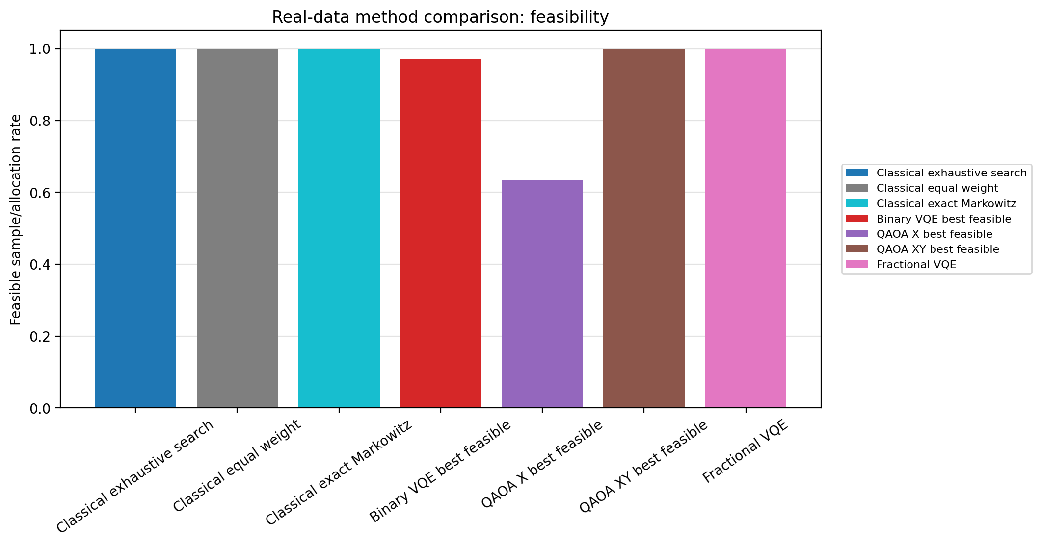
Real-Data Method Comparison

notebooks/Real_Data_Comparison.ipynb writes results/real_data_method_comparison.csv and plots the same-method comparison from those rows. Binary rows use equal-weight selected portfolios for reported return and risk, while objective values remain true binary QUBO objectives. Fractional rows use simplex weights and simplex objectives.

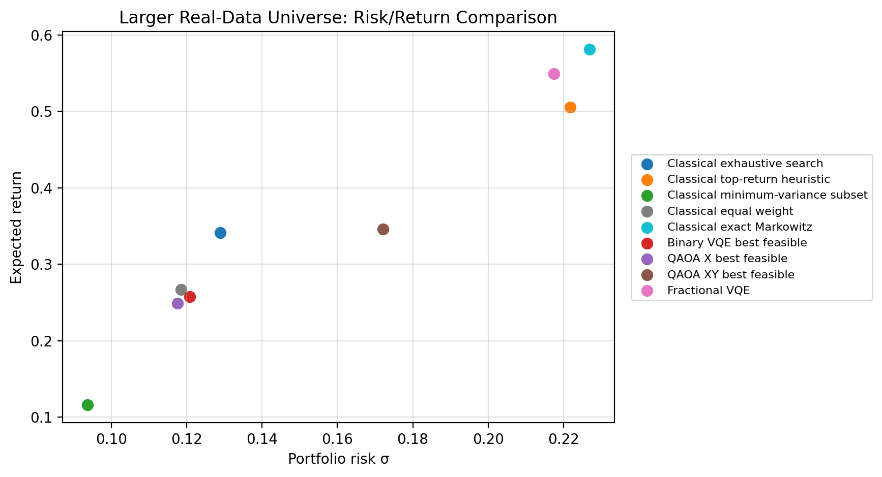
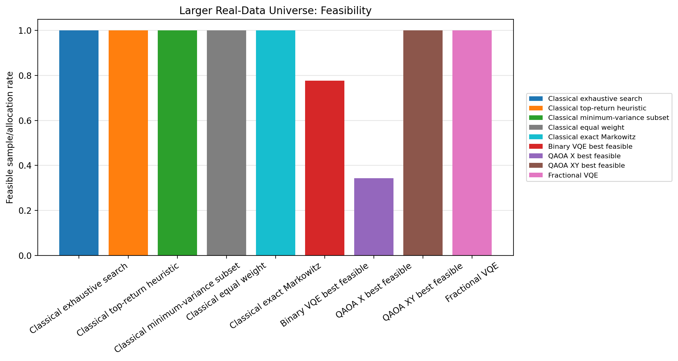
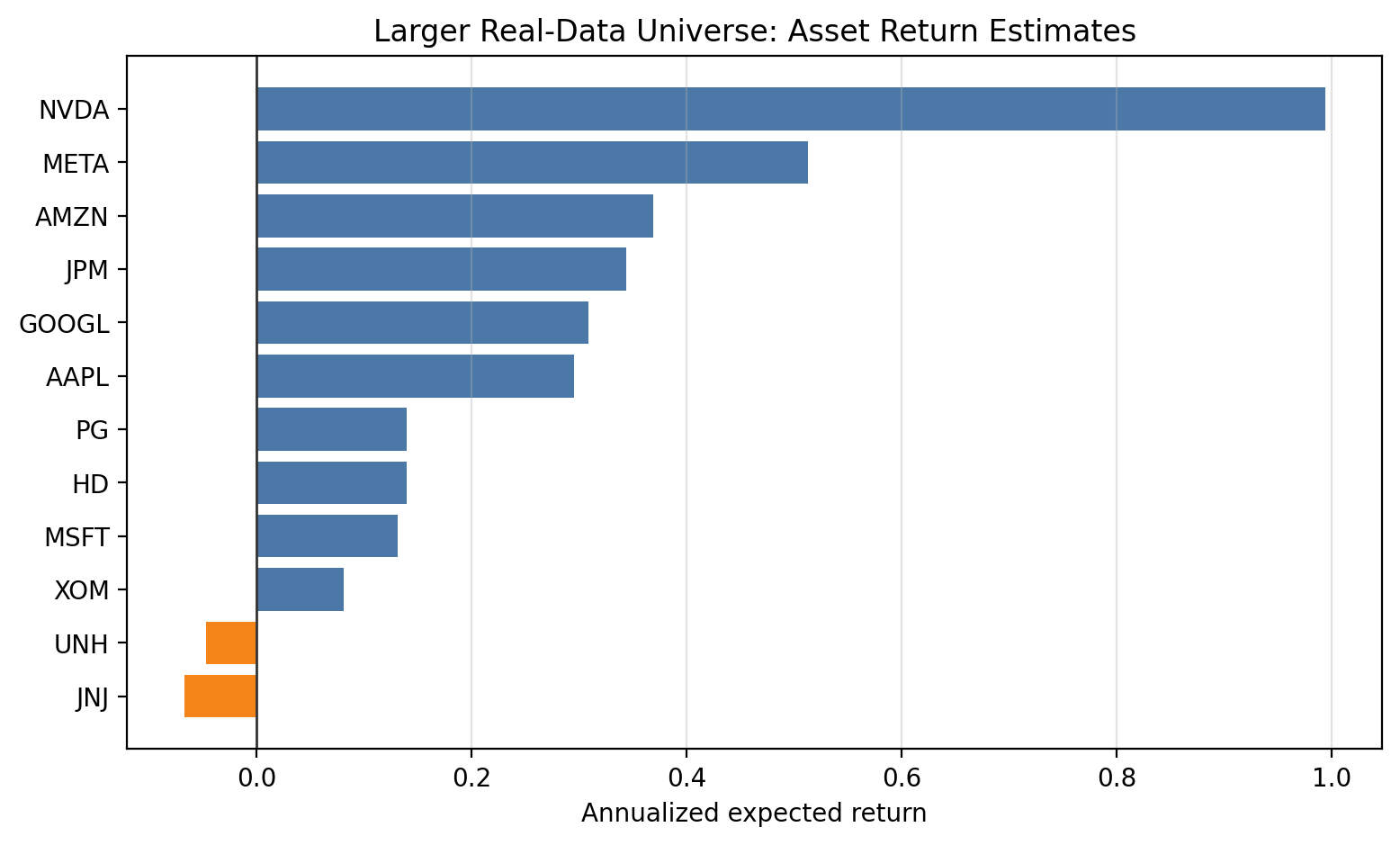
Larger Real-Data Universe

scripts/generate_larger_real_data_example.py writes results/larger_real_data_comparison.csv, regenerates notebooks/examples/04_Larger_Real_Data_Example.ipynb, and saves figures for a 12-stock 2024 market-data window. The binary and QAOA methods use one qubit per asset, so this example is deliberately a scalability/stress example rather than a claim of production scale or quantum advantage.

Regenerate it with:

python scripts/generate_larger_real_data_example.py

Method	Objective family	K	Selection or weights	Return	Risk	Best objective	Feasible rate
Classical exhaustive search	binary QUBO	5	AAPL, NVDA, JPM, JNJ, PG	0.341060	0.128919	-0.043287	1.000000
Binary VQE best feasible	binary QUBO	5	NVDA, XOM, JNJ, PG, HD	0.257295	0.120824	0.173363	0.777344
QAOA X best feasible	binary QUBO	5	AAPL, META, JPM, PG, UNH	0.248903	0.117525	0.136708	0.343750
QAOA XY best feasible	binary QUBO	5	MSFT, NVDA, GOOGL, JPM, UNH	0.346208	0.172098	1.230733	1.000000
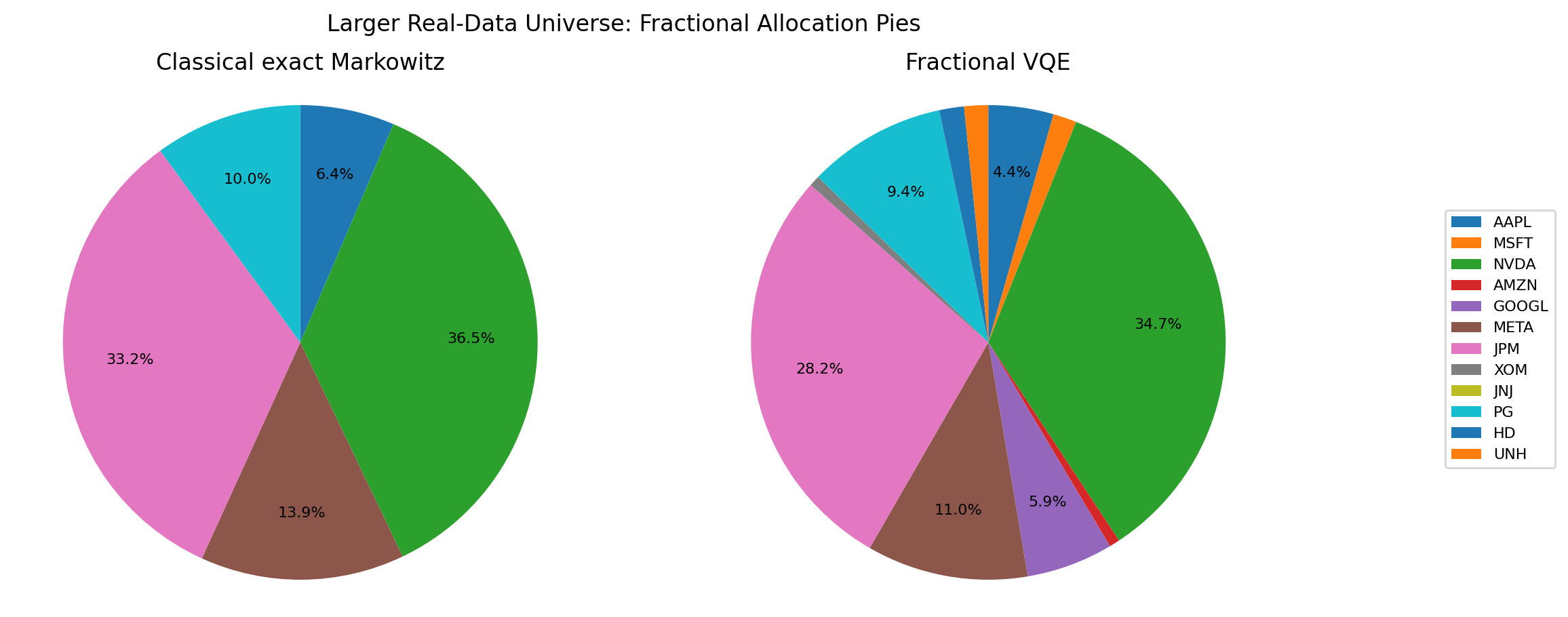
Classical exact Markowitz	fractional simplex		simplex weights	0.580921	0.226857	-0.375066	1.000000
Fractional VQE	fractional simplex		simplex weights	0.549605	0.217478	-0.360419	1.000000

Real Fractional Frontier

Method	λ	Return	Risk
Fractional VQE	8.00	0.324008	0.144192
Fractional VQE	4.00	0.340232	0.151739
Fractional VQE	2.00	0.340300	0.151828
Fractional VQE	1.00	0.340450	0.152215
Fractional VQE	0.50	0.340788	0.153889

Real Binary VQE Figures

Example	Workflow	Figures
notebooks/examples/02_Real_Example.ipynb	Binary VQE	Convergence, probabilities, Top-K selection

Real QAOA Figures

Example	Workflow	Figures
notebooks/examples/03_Real_Example.ipynb	QAOA	Mixer comparison, probabilities, Top-K selections

Real Fractional VQE Figures

Example	Workflow	Figures
notebooks/examples/01_Real_example.ipynb	Fractional VQE	Allocation, frontier, lambda sweep, convergence

Reproducing These Figures

Run the notebooks from the repository root after installing the relevant extras:

pip install -e ".[all]"

Then open the notebook clients:

• notebooks/Binary.ipynb

• notebooks/QAOA.ipynb

• notebooks/Fractional.ipynb

• notebooks/Benchmark_Comparison.ipynb

• notebooks/Real_Data_Comparison.ipynb

• notebooks/Ansatz_Comparison.ipynb

• notebooks/Classical_Markowitz.ipynb

• notebooks/examples/01_Real_example.ipynb

• notebooks/examples/02_Real_Example.ipynb

• notebooks/examples/03_Real_Example.ipynb

• notebooks/examples/04_Larger_Real_Data_Example.ipynb

The notebooks should save updated plots under notebooks/images/ and notebooks/examples/images/.