shors-algorithm-simulation


pip install shors-algorithm-simulation
PyPI
Quantum software portfolio project
A pure Python educational simulator for Shor's period-finding workflow, with explicit matrix mode, faster distribution mode, diagnostics, plots, and a package-ready command line interface.
Install and run
Installable project links with live package metadata badges and direct setup commands.
pip install shors-algorithm-simulation
PyPI
Editable install for tests, examples, and local documentation builds.
python -m pip install -e ".[test]"
GitHub
Optional dependencies for Qiskit circuit diagram generation.
python -m pip install ".[circuits]"
Circuits
Documentation map
- [Intro](#intro) - [Classical Pre-Processing](#classical-pre-processing) - [Quantum Period Finding](#quantum-period-finding) - [Registers](#registers) - [Hadamard...
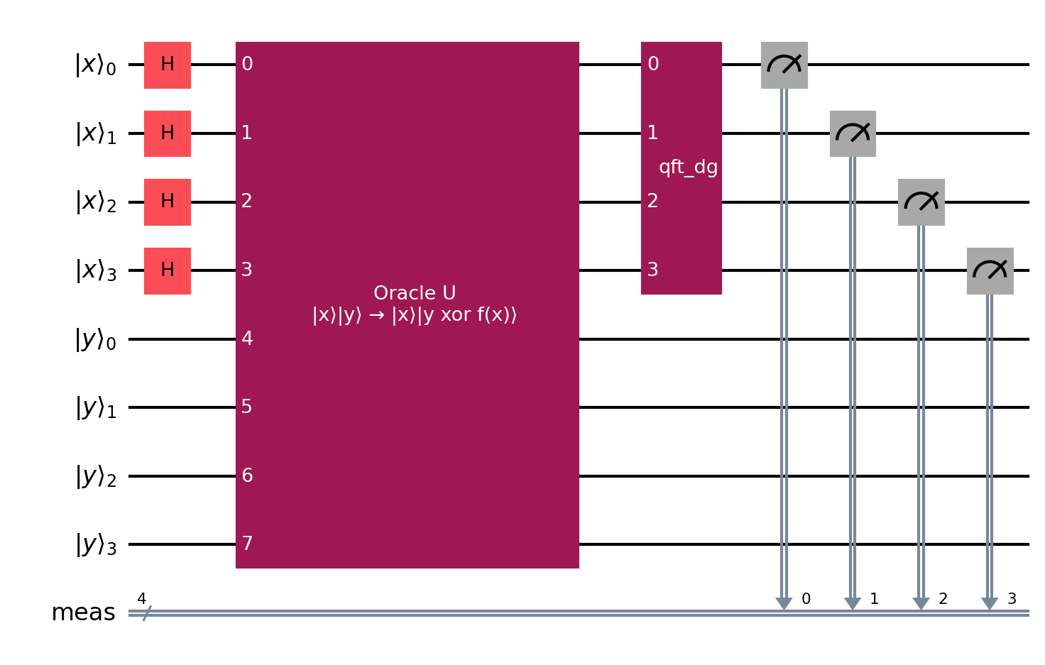
This file explains the circuit diagrams generated by the repository. It keeps one drawing for each concept:
For $N=35$ and $a=2$, the multiplicative order of $a \bmod N$ is $r=12$. This is a useful Shor period because it is even and it produces non-trivial factors in the final...
All notable changes to this project are documented here.
Complete README


Project website: https://SidRichardsQuantum.github.io/Shors_Algorithm_Simulation/
PyPI: https://pypi.org/project/shors-algorithm-simulation/
A pure Python implementation of Shor's quantum factorization algorithm using classical simulation of the period-finding step. The project supports both explicit matrix simulation for very small inputs and a faster distribution-based simulation for the ideal first-register measurement probabilities.
Shor's algorithm is a quantum algorithm that efficiently finds the prime factors of large integers, which forms the basis for breaking RSA encryption.
This implementation simulates the quantum operations classically to illustrate how Shor's algorithm works step by step. mode="matrix" explicitly applies the simulated gates and grows exponentially in memory; mode="distribution" computes the same ideal first-register probability distribution without materializing the full matrices.
See the theory walkthrough for a descriptive algorithm walkthrough.
See the circuit walkthrough for the register and circuit-diagram walkthrough.
See the results page for results and conclusions.
Q ~= N^2 and a function register large enough to store values modulo Na^x mod N in a reversible oracle to entangle the registersA quantum circuit sketch for Shor's Algorithm using 8 qubits:
shots sampling draws stochastic first-register measurements from the ideal distributionmax_attempts can try multiple bases when a is not providedmode="distribution" computes the ideal first-register measurement distribution directly, using the standard Q ~= N^2 period register size.mode="matrix" explicitly applies the simulated Hadamard, oracle, and IQFT matrices for very small inputs.shors_algorithm_simulation/
Core API, CLI, validation, probability distributions, period recovery, plotting helpers, and quantum operator modules.
examples/
Runnable factorisation demos, no-plot runs, shot sweeps, diagnostics, runtime benchmarks, and circuit diagram generation.
README.md, THEORY.md, CIRCUITS.md, RESULTS.md, CHANGELOG.md
Pages source files rendered into the static GitHub Pages site.
images/
Probability plots, oracle-period diagnostics, continued-fraction outputs, circuit diagrams, and runtime visualizations.
tests/
Regression tests for CLI behavior, period finding, circuit diagram support, and installation smoke checks.
pyproject.toml, scripts/build_pages.py, .github/workflows/
Package metadata, local/static documentation builder, test workflow, Pages deployment, and PyPI publishing automation.
python -m pip install shors-algorithm-simulation
The PyPI install command applies after the first published release.
For development from source:
git clone https://github.com/SidRichardsQuantum/Shors_Algorithm_Simulation
cd Shors_Algorithm_Simulation
python -m pip install -e ".[test]"
Circuit diagram generation uses optional Qiskit dependencies:
python -m pip install ".[circuits]"
Terminal inputs:
python -m examples.factorisation_example   # single run with plot output
python -m examples.no_plot_example         # single run without plotting
python -m examples.multiple_cases_example  # batch of small deterministic cases
python -m examples.shots_sweep_example     # plot success rate vs sampled shots
python -m examples.visualizations_example  # generate educational diagnostic plots
python -m examples.circuit_diagrams_example --N 15 --a 2
Command-line usage:
shors-sim --N 35 --a 2 --mode distribution --plots --output-dir images
shors-sim --N 15 --a 2 --mode matrix --json
shors-sim --N 21 --a 2 --shots 1024 --seed 1 --json
shors-sim --N 33 --max-attempts 5 --seed 0
python main.py ... is kept as a compatibility entry point for running from a source checkout.
Visualization plots can also be selected from the command line:
python -m examples.shots_sweep_example --N 21 --a 2 --shots 16 32 64 128 256 --trials 20
python -m examples.visualizations_example --N 35 --a 2 --plots oracle marked continued
python -m examples.visualizations_example --plots comparison --comparison-N 15 --comparison-a 2
Circuit diagrams can be generated from the command line:
python -m examples.circuit_diagrams_example --N 15 --a 2 --output-dir images
python -m shors_algorithm_simulation.quantum.circuits --N 35 --a 2
Programmatic mode selection:
from shors_algorithm_simulation import shors_simulation

result = shors_simulation(N=21, a=2, mode="distribution")
print(result["success"], result["factors"], result["period"])

matrix_result = shors_simulation(N=15, a=2, mode="matrix")
print(matrix_result["success"], matrix_result["factors"], matrix_result["period"])

sampled_result = shors_simulation(N=21, a=2, shots=1024, random_seed=1)
print(sampled_result["measurement_counts"])

retry_result = shors_simulation(N=33, max_attempts=5, random_seed=0)
print(retry_result["success"], len(retry_result["attempts"]))
distribution mode is the default and is appropriate for the documented examples. matrix mode is intended for the smallest cases because explicit gate matrices grow quickly.
shors_simulation returns a dictionary containing success, N, a, mode, period, factors, message, classical_precheck, shots, measurement_counts, and attempts.
Output:
N = 35
Attempt 1: a = 2
The period r = 12 is even.
a^(r/2) + 1 = 30, and gcd(30, 35) = 5
a^(r/2) - 1 = 28, and gcd(28, 35) = 7
The factors of N = 35 are 5 and 7.
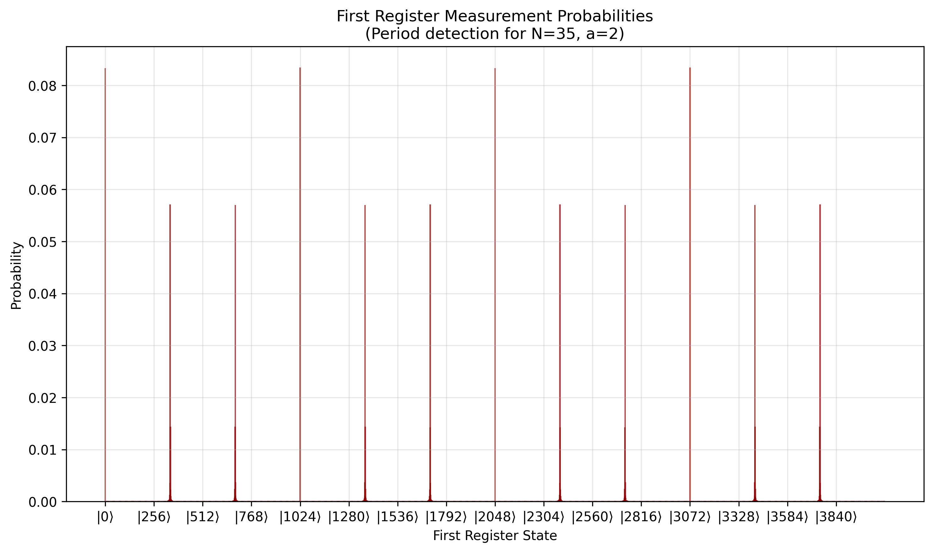
This also saves the plot to the "images" directory as "first_register_probabilities_N=35_a=2.png":
examples/visualizations_example.py generates:
x -> a^x mod Nexamples/shots_sweep_example.py repeats sampled period recovery for multiple shot counts and saves a CSV plus a success-rate plot. It is intended to show how empirical measurement histograms converge toward the ideal distribution as shots increase.
mode="matrix" constructs the full simulated state evolution for tiny examples, so it is useful for checking the gate-level model but grows quickly.
mode="distribution" computes the ideal post-IQFT first-register probability distribution directly from the periodic oracle values. It does not build a scalable quantum computer or simulate hardware noise.
When shots is provided, the simulator samples measurement counts from that ideal distribution and then runs the same continued-fraction recovery on the empirical histogram.
python -m pytest -q
ruff check .
black --check .
Releases are published to PyPI by GitHub Actions trusted publishing when a GitHub Release is published with a tag matching the version in pyproject.toml.
mode="matrix" scales exponentially with the number of simulated qubits and is only practical for tiny cases.mode="distribution" avoids full matrices by computing the ideal first-register distribution directly, which is still a classical simulation of the period-finding output.shots samples from the ideal distribution; it does not model device noise, decoherence, or imperfect gates.QFTGate APIcircuit_drawer APIFraction.limit_denominatorsavefigThis implementation is inspired by the original work of Peter Shor and serves as an educational tool for understanding quantum algorithms through classical simulation.
Note: This is a classical simulation for educational purposes. Real quantum advantage requires actual quantum hardware that can efficiently implement this factorisation algorithm in polynomial time (commonly cited as roughly $O((\log N)^3)$ for idealized gate complexity).
Sid Richards
MIT. See LICENSE.