Results

Detailed Example: N=35, a=2

For $N=35$ and $a=2$, the multiplicative order of $a \bmod N$ is $r=12$. This is a useful Shor period because it is even and it produces non-trivial factors in the final classical post-processing step.

The powers of $2 \bmod 35$ repeat after 12 steps:

2^0  mod 35 = 1
2^1  mod 35 = 2
2^2  mod 35 = 4
2^3  mod 35 = 8
2^4  mod 35 = 16
2^5  mod 35 = 32
2^6  mod 35 = 29
2^7  mod 35 = 23
2^8  mod 35 = 11
2^9  mod 35 = 22
2^10 mod 35 = 9
2^11 mod 35 = 18
2^12 mod 35 = 1

The oracle-period plot shows this hidden periodic function before the IQFT is applied:

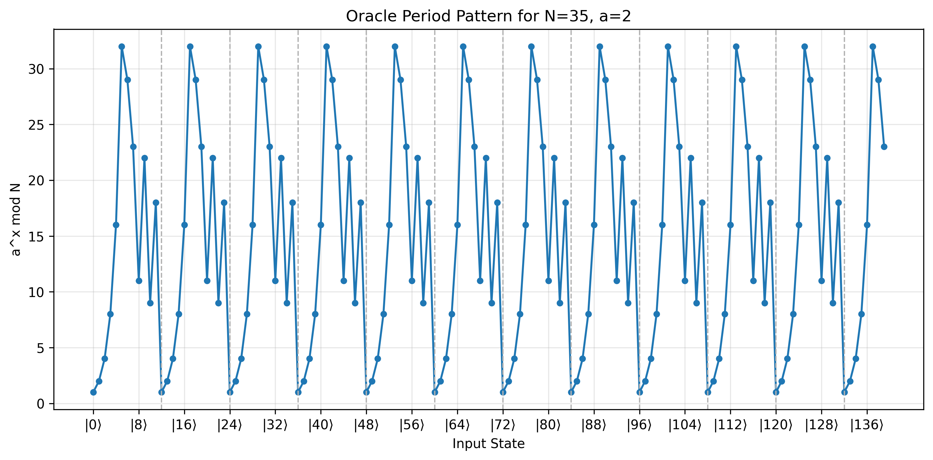
Each vertical repeat corresponds to the same modular value appearing again ($12$ peaks corresponding to a period of $12$). This repeated structure is what the quantum Fourier transform converts into measurement peaks.

First-Register Probability Distribution

For $N=35$, the simulator uses:

n = ceil(log2(35)) = 6
Q = 2^(2n) = 4096

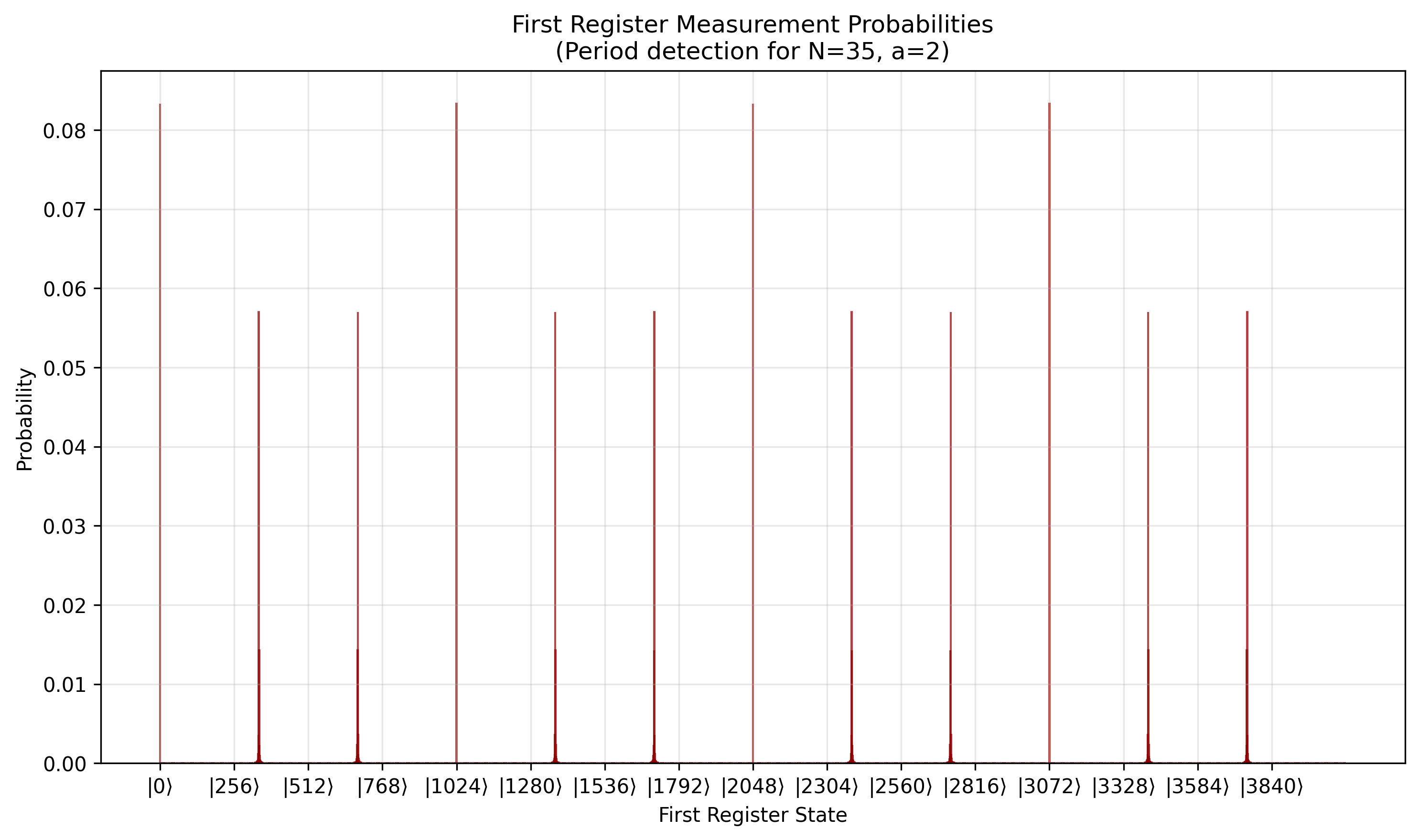
After the oracle and IQFT, first-register probabilities concentrate near states satisfying:

c / Q ~= s / r

where s is an integer. Since $r=12$, the expected peak spacing is approximately:

Q / r = 4096 / 12 = 341.33...

So high-probability states should appear near:

|0⟩, |341⟩, |683⟩, |1024⟩, |1365⟩, |1707⟩, ...

The marked probability plot overlays these expected peak locations for the recovered period:

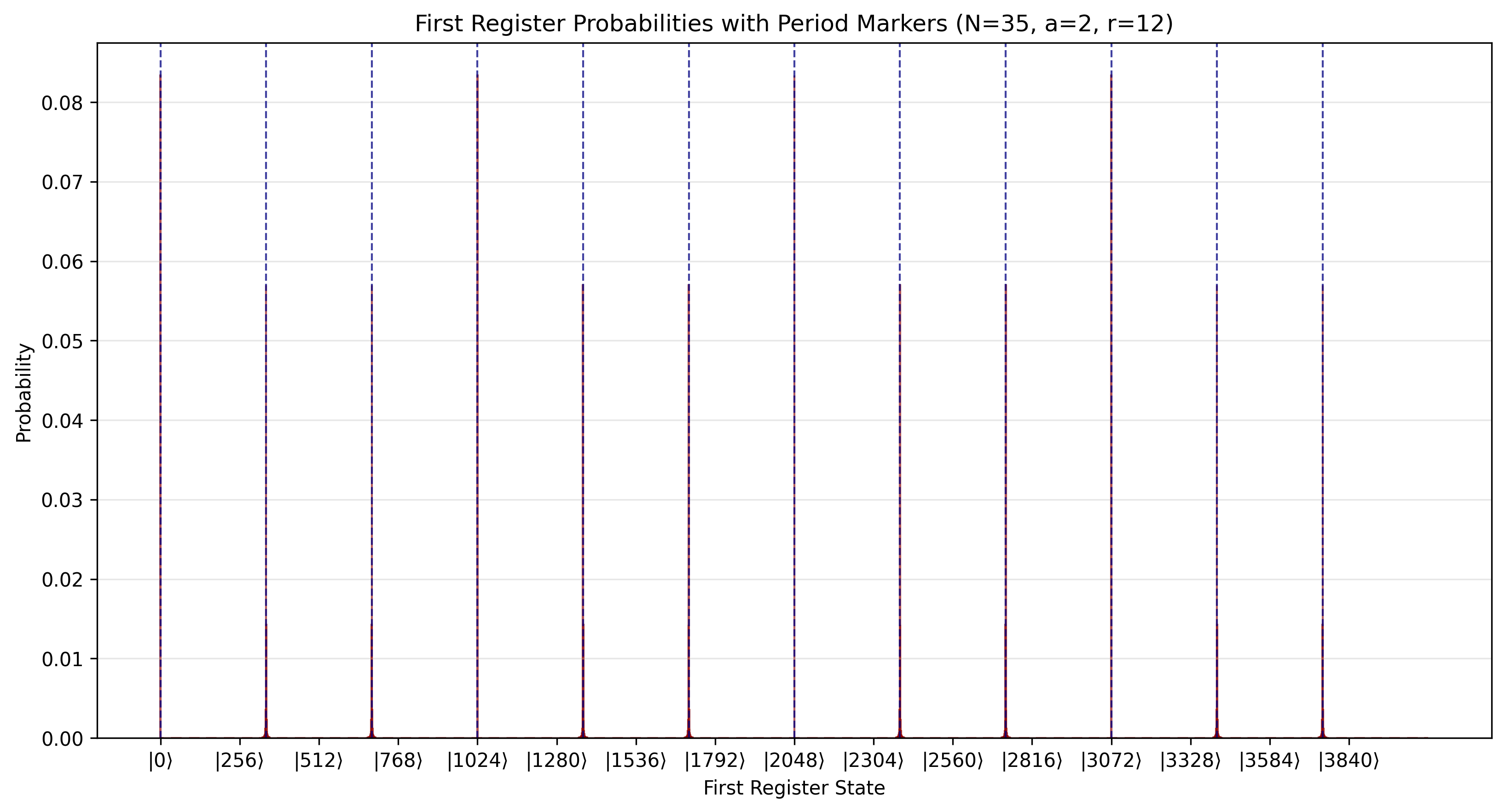
The peaks are not all exactly equally high because $4096$ is not divisible by $12$. That mismatch is expected: the IQFT concentrates probability near the closest integer states to $sQ/r$, not always exactly on them.

Running:

from shors_algorithm_simulation import shors_simulation

shors_simulation(N=35, a=2, sparse=True, mode="distribution")

prints:

N = 35
Attempt 1: a = 2
The period r = 12 is even.
a^(r/2) + 1 = 30, and gcd(30, 35) = 5
a^(r/2) - 1 = 28, and gcd(28, 35) = 7
The factors of N = 35 are 5 and 7.

The function also returns a structured result dictionary containing the recovered period and factors.

Continued-Fraction Recovery

The period finder does not count peaks directly. It sorts measurement outcomes by probability, turns each outcome c into the fraction c / Q, and uses continued fractions to recover denominator candidates.

For $N=35, a=2$, several of the highest-probability measured states immediately point to period candidates related to $12$:

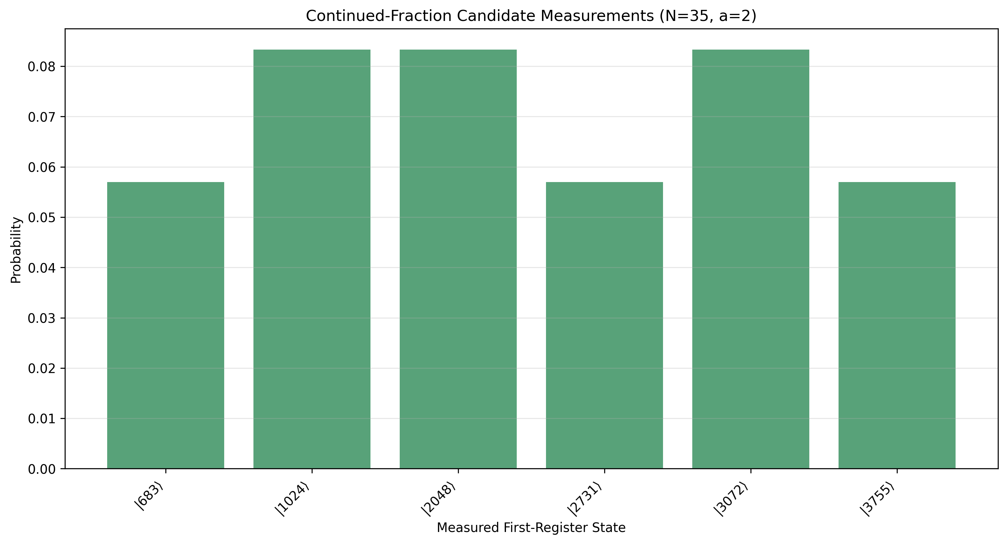
Some measured values produce denominators such as 2, 4, or 6, which are divisors of the true period rather than the full period. The implementation therefore tests the denominator and its multiples. In this run, the validated useful period is $r=12$.

A candidate period is accepted only when it can actually produce non-trivial factors:

pow(a, r, N) == 1
1 < gcd(a^(r/2) - 1, N) < N
1 < gcd(a^(r/2) + 1, N) < N

The diagnostic plot highlights the continued-fraction candidates that lead to an accepted period:

The same diagnostics are also saved as a CSV file:

images/continued_fraction_candidates_N=35_a=2.csv

Factor Extraction for N=35, a=2

Once the period is recovered, the final step is entirely classical. Since $r=12$:

r / 2 = 6
2^6 = 64
64 mod 35 = 29

Now compute:

gcd(2^6 - 1, 35) = gcd(63, 35) = gcd(28, 35) = 7
gcd(2^6 + 1, 35) = gcd(65, 35) = gcd(30, 35) = 5

So the non-trivial factors are:

35 = 5 * 7

Retry Case: N=33, a=2

Some choices of a have a valid period but still do not produce non-trivial factors. For example, $N=33, a=2$ has true order $r=10$, but:

2^(10/2) == -1 (mod 33)

This makes the factor extraction step trivial, so Shor's algorithm should be retried with a different base. The simulator now reports this as an expected retry rather than returning incorrect factors.

Using $a=5$ for $N=33$ succeeds and recovers factors $3$ and $11$.

Additional Visualizations and Mode Comparison

examples/visualizations_example.py generates a set of educational plots.

For tiny examples, matrix mode and distribution mode can be compared directly:

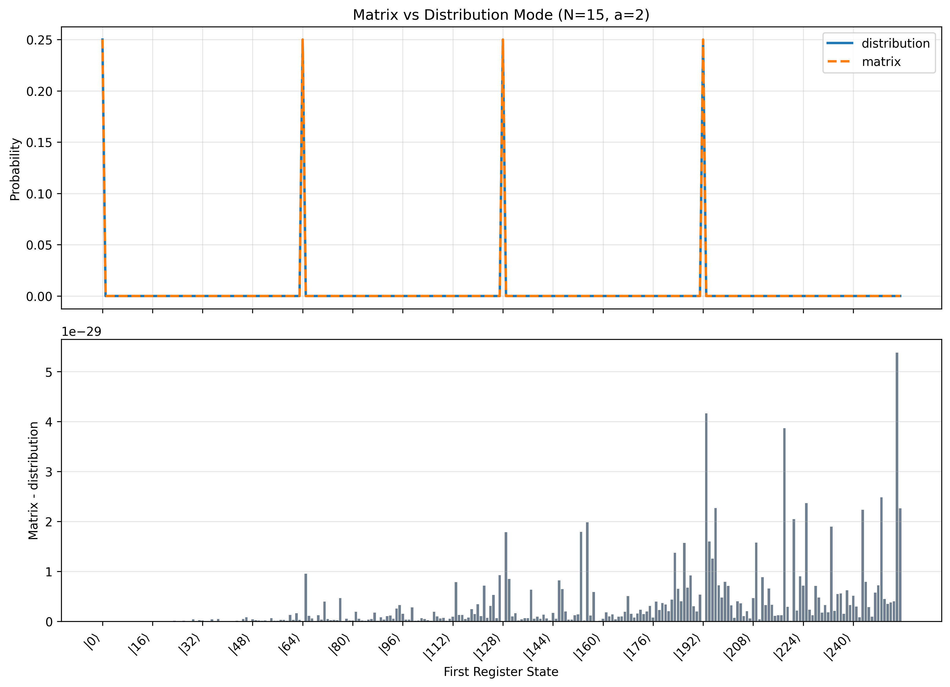
The two distributions match up to floating-point error for $N=15, a=2$.

Runtimes Vs Required Qubits

Running python -m examples.runtimes_test calls run_runtime_analysis() from shors_algorithm_simulation.plotting.runtime. It measures repeated runtimes for deterministic pairs (N, a) known to yield useful periods.

Example cases include:

(15, 2)   # 3 * 5
(21, 2)   # 3 * 7
(33, 5)   # 3 * 11
...
(141, 2)  # 3 * 47
(161, 6)  # 7 * 23

Runtimes are plotted against $N$ and against the simulated qubit count. Current runtime plots include the simulation mode in the filename.

The checked-in runtime plot below was generated from a short deterministic subset:

(15, 2)
(21, 2)
(33, 5)
(35, 2)

images/runtime_vs_qubit_sparse_True_mode_distribution_repeats_3.png

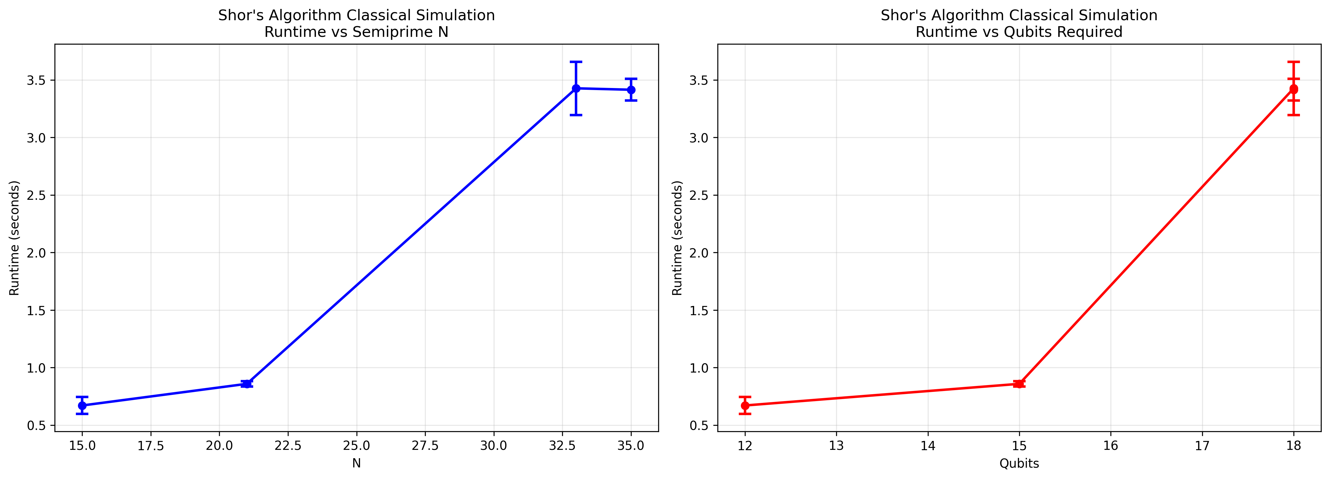
The explicit matrix mode grows quickly because it materializes operators over the full simulated Hilbert space. Distribution mode is faster because it computes the ideal first-register measurement distribution directly, but it remains a classical educational simulation rather than a scalable factoring implementation.

References

• Peter W. Shor, "Polynomial-Time Algorithms for Prime Factorization and Discrete Logarithms on a Quantum Computer" (arXiv)
• IBM Quantum tutorial: Shor's algorithm
• Python Fraction.limit_denominator
• NumPy inverse FFT
• Matplotlib savefig

Author

Sid Richards

• LinkedIn: sid-richards-21374b30b
• GitHub: SidRichardsQuantum

License

MIT. See LICENSE.