Benchmark Results
This generated page displays embedded benchmark plots and text outputs from the classical-baseline benchmark notebooks.
Current Status
Source notebooks:
notebooks/benchmarks/Notebooks displayed:
4Embedded plot artefacts displayed:
8Plain-text notebook results displayed:
6Plot manifest:
results/tables/benchmark_plot_manifest.csv
Regeneration
Execute notebooks, extract their embedded outputs, and refresh this page with:
python scripts/extract_notebook_plots.py --preset benchmarks --execute --write-docs
Notebook Results
01_linear_system_classical_vs_qsvt_proxy.ipynb
Source: notebooks/benchmarks/01_linear_system_classical_vs_qsvt_proxy.ipynb
Output 1 (cell 7):
Poisson system
--------------
Dimension : 12
Condition number : 67.83
Scaled spectral gap gamma : 0.01474
Inverse polynomial degree : 9
Output 2 (cell 11):
Benchmark readout
-----------------
Dense relative residual : 2.78e-15
CGS relative residual : 7.68e-15
CGS iterations : 1
QSVT signal calls : 9
02_matrix_functions_spectral_baselines.ipynb
Source: notebooks/benchmarks/02_matrix_functions_spectral_baselines.ipynb
Output 1 (cell 8):
Matrix-function benchmark readout
---------------------------------
Spectral baseline problem   : exponential-matrix-function
Thermal polynomial degree : 10
Filter polynomial degree : 10
Filter QSVT signal calls : 10
03_scaling_sweeps.ipynb
Source: notebooks/benchmarks/03_scaling_sweeps.ipynb
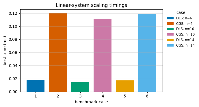
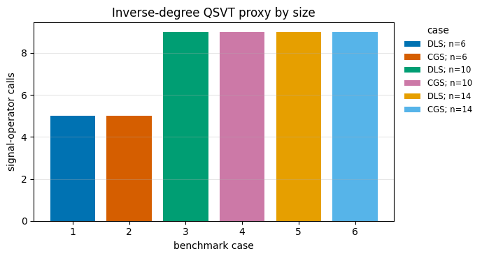
Output 1 (cell 8):
Scaling sweep readout
---------------------
Reports : 6
Matrix dimensions : 6, 10, 14
Max QSVT signal calls : 9
04_classical_baseline_assumptions.ipynb
Source: notebooks/benchmarks/04_classical_baseline_assumptions.ipynb
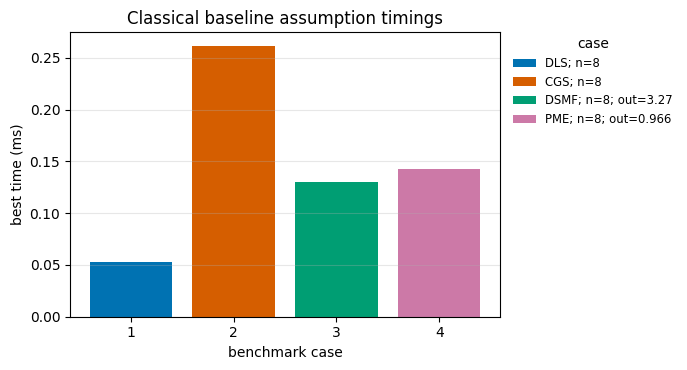
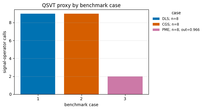
Output 1 (cell 8):
Linear-system baseline readout
==============================
Case Classical algorithm Condition Relative residual QSVT degree [polynomial degree] Signal calls [operator calls]
---- ---------------------------------------- --------- ----------------- ------------------------------- -----------------------------
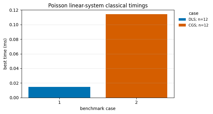
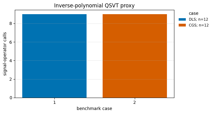
DLS numpy.linalg.solve 4 8.86e-17 9 9
CGS qsvt.benchmarks.conjugate_gradient_solve 4 1.77e-16 9 9
DLS times a dense direct solve. CGS reports iterative-solver diagnostics, but this educational benchmark still uses dense NumPy matrix-vector products.
Output 2 (cell 10):
Matrix-function baseline readout
================================
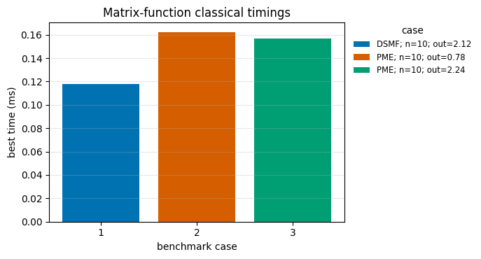
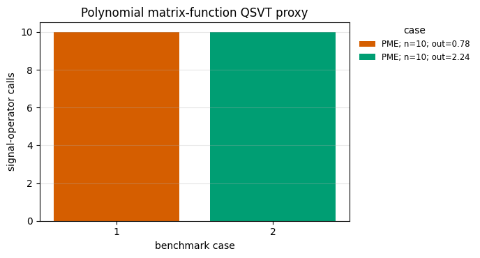
Case Classical algorithm QSVT degree [polynomial degree] Signal calls [operator calls] Best time (s)
---- ------------------------------ ------------------------------- ----------------------------- -------------
DSMF dense-spectral-matrix-function n/a n/a 1.30e-04
PME spectral-polynomial-evaluation 2 2 1.43e-04
DSMF is the exact dense spectral reference. PME applies the supplied polynomial classically and is the closest fixed-polynomial comparison to a QSVT sequence.