Tutorial Results
This generated page displays the embedded plots and text outputs from every tutorial notebook.
Current Status
Source notebooks:
notebooks/tutorials/Notebooks displayed:
19Embedded plot artefacts displayed:
38Plain-text notebook results displayed:
81
Regeneration
Execute notebooks, extract their embedded outputs, and refresh this page with:
python scripts/extract_notebook_plots.py --preset tutorials --execute --write-docs
Notebook Results
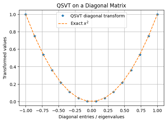
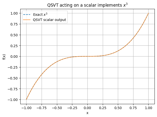
01_QSVT_Scalar_and_Diagonal_Matrix.ipynb
Source: notebooks/tutorials/01_QSVT_Scalar_and_Diagonal_Matrix.ipynb
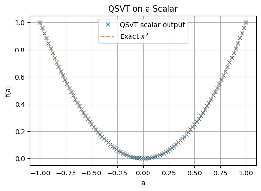
Output 1 (cell 6):
coeffs = [0. 0. 1.]
x_demo = [-1.  -0.5  0.   0.5  1. ]
f(x_demo) = [1.   0.25 0.   0.25 1.  ]
Output 2 (cell 11):
a0 = 0.6
QSVT output = 0.3599999999996402
Exact f(a0) = 0.36
Absolute error = 3.598e-13
Output 3 (cell 17):
scalar_abs_error: 3.598e-13
diagonal_max_error: 1.000e-12
validation: passed
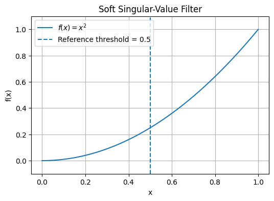
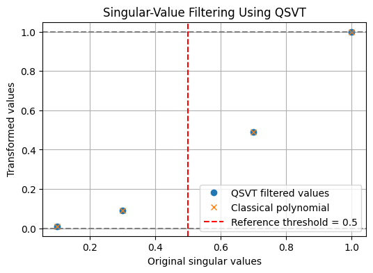
02_QSVT_Singular_Value_Filter.ipynb
Source: notebooks/tutorials/02_QSVT_Singular_Value_Filter.ipynb
Output 1 (cell 4):
A = [[1.  0.  0.  0. ]
 [0.  0.7 0.  0. ]
 [0.  0.  0.3 0. ]
 [0.  0.  0.  0.1]]
Output 2 (cell 6):
Filter coefficients: [0. 0. 1.]
Bounded on [-1,1]: True
Output 3 (cell 8):
Original singular values: [1.  0.7 0.3 0.1]
Transformed singular values: [1.   0.49 0.09 0.01]
Output 4 (cell 13):
Comparison helper output
------------------------
Input σ | QSVT output | Classical output | abs. error
------- | ----------- | ---------------- | ----------
1 | 1 | 1 | 1.00e-12
0.7 | 0.49 | 0.49 | 4.90e-13
0.3 | 0.09 | 0.09 | 8.98e-14
0.1 | 0.01 | 0.01 | 9.83e-15
Output 5 (cell 15):
max_abs_error: 1.000e-12
transformed_singular_values: [1.   0.49 0.09 0.01]
validation: passed
03_QSP_Polynomial_Demo.ipynb
Source: notebooks/tutorials/03_QSP_Polynomial_Demo.ipynb
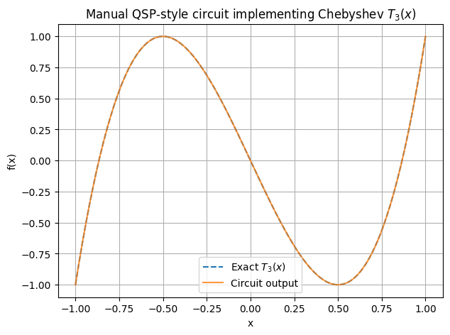
Output 1 (cell 10):
qsvt_scan_max_error: 9.999e-13
circuit_max_error: 7.216e-16
validation: passed
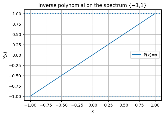
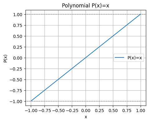
04_QSVT_Linear_Solver_2x2.ipynb
Source: notebooks/tutorials/04_QSVT_Linear_Solver_2x2.ipynb
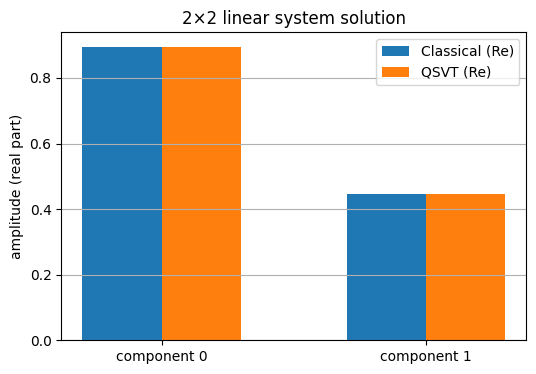
Output 1 (cell 4):
A = [[0. 1.]
 [1. 0.]]

b = [1. 2.]

Classical solution: [2. 1.]

Normalized classical solution: [0.89442719 0.4472136 ]

Eigenvalues of A: [-1.  1.]
Output 2 (cell 6):
Polynomial coefficients: [0. 1.]
Parity [polynomial parity]: odd
Output 3 (cell 9):
QSVT top-left block P(A):
[[0.+0.e+00j 1.+1.e-06j]
 [1.+1.e-06j 0.+0.e+00j]]

Direct A:
[[0. 1.]
 [1. 0.]]
Output 4 (cell 12):
execution_kind: pennylane-qnode-statevector-qsvt-execution
gate_types: {'StatePrep': 1, 'QSVT': 1}
logical_success_probability: 1.000000000000
QNode QSVT solution (normalized): [0.89442719+1.26489707e-06j 0.4472136 +6.32448537e-07j]

Classical solution (normalized): [0.89442719 0.4472136 ]
Output 5 (cell 17):
block_max_error: 1.414e-06
solution_overlap: 1.000000000000
validation: passed
05_QSVT_Linear_Solver_4x4.ipynb
Source: notebooks/tutorials/05_QSVT_Linear_Solver_4x4.ipynb
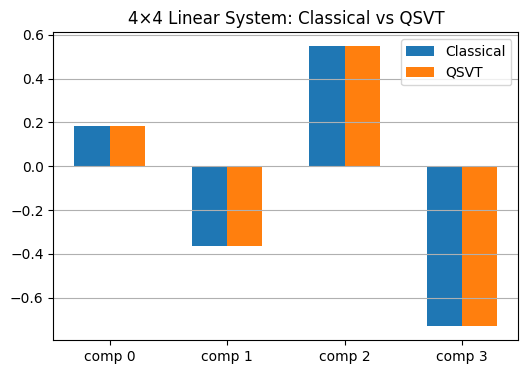
Output 1 (cell 4):
A = [[ 1.  0.  0.  0.]
 [ 0. -1.  0.  0.]
 [ 0.  0.  1.  0.]
 [ 0.  0.  0. -1.]]

Eigenvalues: [-1. -1.  1.  1.]

b = [1. 2. 3. 4.]

Classical x = [ 1. -2.  3. -4.]

Classical (normalized) = [ 0.18257419 -0.36514837  0.54772256 -0.73029674]
Output 2 (cell 6):
Polynomial coefficients: [0. 1.]
Parity [polynomial parity]: odd
Output 3 (cell 9):
QSVT top-left block P(A):
[[ 1.+1.e-06j  0.+0.e+00j  0.+0.e+00j  0.+0.e+00j]
 [ 0.+0.e+00j -1.-1.e-06j  0.+0.e+00j  0.+0.e+00j]
 [ 0.+0.e+00j  0.+0.e+00j  1.+1.e-06j  0.+0.e+00j]
 [ 0.+0.e+00j  0.+0.e+00j  0.+0.e+00j -1.-1.e-06j]]

Direct A:
[[ 1.  0.  0.  0.]
 [ 0. -1.  0.  0.]
 [ 0.  0.  1.  0.]
 [ 0.  0.  0. -1.]]
Output 4 (cell 12):
execution_kind: pennylane-qnode-statevector-qsvt-execution
gate_types: {'StatePrep': 1, 'QSVT': 1}
logical_success_probability: 1.000000000000
QNode QSVT solution (normalized) = [ 0.18257419+2.58196034e-07j -0.36514837-5.16392068e-07j
  0.54772256+7.74588102e-07j -0.73029674-1.03278414e-06j]
Classical solution (normalized) = [ 0.18257419 -0.36514837  0.54772256 -0.73029674]
Output 5 (cell 16):
block_max_error: 1.414e-06
solution_overlap: 1.000000000000
validation: passed
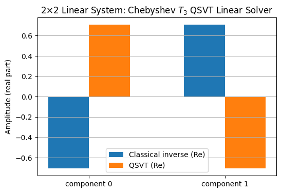
06_QSVT_Linear_Solver_Approximate.ipynb
Source: notebooks/tutorials/06_QSVT_Linear_Solver_Approximate.ipynb
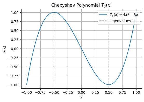
Output 1 (cell 4):
A = [[-0.5  0. ]
 [ 0.   0.5]]
Eigenvalues of A: [-0.5  0.5]
b = [0.70710678 0.70710678]
True inverse solution x_true = A^{-1} b = [-1.41421356  1.41421356]
True inverse solution (normalized) = [-0.70710678  0.70710678]
Output 2 (cell 8):
Polynomial coefficients: [ 0. -3.  0.  4.]
Polynomial degree [polynomial degree]: 3
Polynomial parity [polynomial parity]: odd
Bounded on [-1,1]: True

T3(-0.5) = 1.0
T3( 0.5) = -1.0

Inverse eigenvalues 1/lambda: [-2.  2.]

Ratio T3(lambda0) / T3(lambda1) = -1.0
Ratio (1/lambda0) / (1/lambda1) = -1.0
Output 3 (cell 12):
QSVT top-left block P(A):
[[ 1.+1.e-06j  0.+0.e+00j]
 [ 0.+0.e+00j -1.-1.e-06j]]

Direct P(A):
[[ 1.  0.]
 [ 0. -1.]]
Output 4 (cell 15):
execution_kind: pennylane-qnode-statevector-qsvt-execution
gate_types: {'StatePrep': 1, 'QSVT': 1}
logical_success_probability: 1.000000000000
QNode QSVT solution (normalized) = [ 0.70710678+9.99988939e-07j -0.70710678-9.99988939e-07j]
True inverse solution (normalized) = [-0.70710678  0.70710678]
Output 5 (cell 19):
block_max_error: 1.414e-06
solution_direction_overlap: 1.000000000000
validation: passed
07_QSVT_Polynomial_Design_and_Approximation.ipynb
Source: notebooks/tutorials/07_QSVT_Polynomial_Design_and_Approximation.ipynb
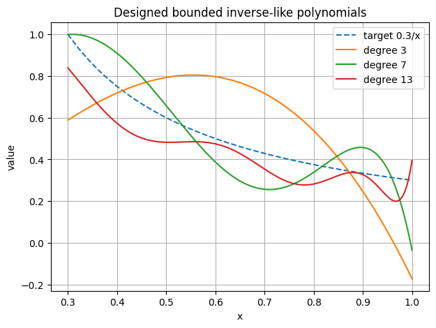
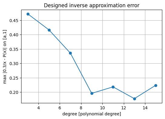
Output 1 (cell 13):
best_degree [polynomial degree]: 13
best_inverse_error: 1.775e-01
max_bounded_value: 1.000000
validation: passed
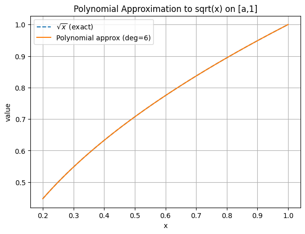
08_QSVT_Matrix_Functions_Powers_and_Roots.ipynb
Source: notebooks/tutorials/08_QSVT_Matrix_Functions_Powers_and_Roots.ipynb
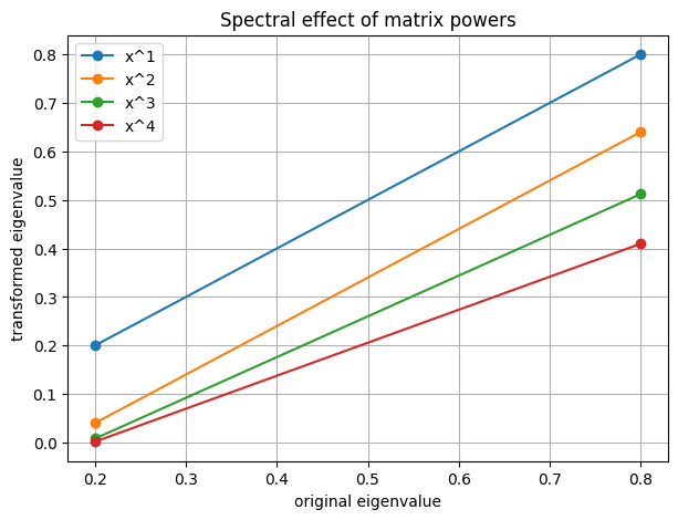
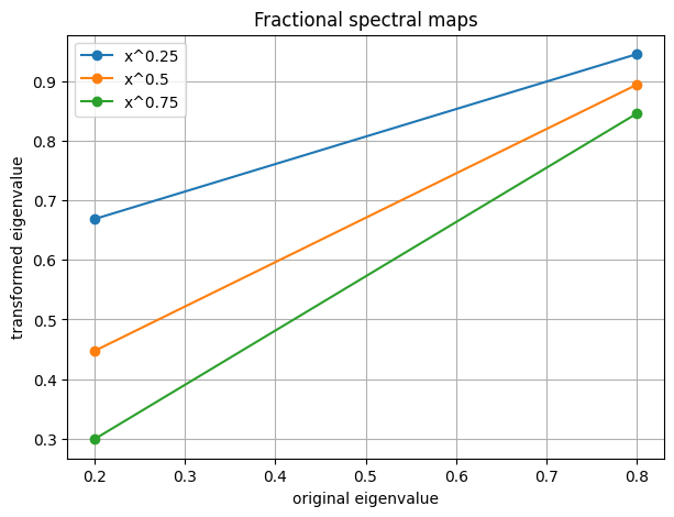
Output 1 (cell 4):
A = [[ 0.391293 -0.279612]
 [-0.279612  0.608707]]

Eigenvalues = [0.2 0.8]
Output 2 (cell 7):
A^2 via spectral map:
[[ 0.231293 -0.279612]
 [-0.279612  0.448707]]
Output 3 (cell 9):
Bounded on [a,1] [boolean]: True
Output 4 (cell 12):
sqrt(A) exact:
[[ 0.589795 -0.20841 ]
 [-0.20841   0.751846]]

sqrt(A) polynomial:
[[ 0.589848 -0.208365]
 [-0.208365  0.751864]]
Output 5 (cell 15):
A^0.5 via spectral routine:
[[ 0.589795 -0.20841 ]
 [-0.20841   0.751846]]
Output 6 (cell 18):
sqrt_poly_max_error: 5.293e-05
spectral_square_error: 3.331e-16
validation: passed
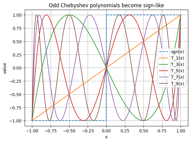
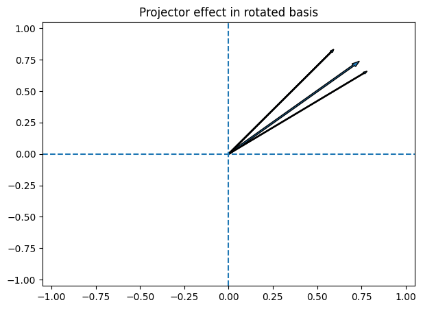
09_QSVT_Sign_Function_and_Projectors.ipynb
Source: notebooks/tutorials/09_QSVT_Sign_Function_and_Projectors.ipynb
Output 1 (cell 5):
Parity [polynomial parity]: odd
Bounded [boolean]: True
Output 2 (cell 7):
Degree  1 → [0.316228 0.948683]
Degree  3 → [1. 0.]
Degree  5 → [0.316228 0.948683]
Degree  7 → [0.316228 0.948683]
Degree  9 → [1. 0.]
Output 3 (cell 9):
A = [[-0.08498357 -0.49272486]
 [-0.49272486  0.08498357]]

Eigenvalues = [-0.5  0.5]
Output 4 (cell 12):
Positive projector:
[[ 0.415016 -0.492725]
 [-0.492725  0.584984]]

Negative projector:
[[0.584984 0.492725]
 [0.492725 0.415016]]
Output 5 (cell 15):
projector_completeness_error: 0.000e+00
positive_projector_trace [states]: 1.000000
validation: passed
10_QSVT_Design_and_Templates.ipynb
Source: notebooks/tutorials/10_QSVT_Design_and_Templates.ipynb
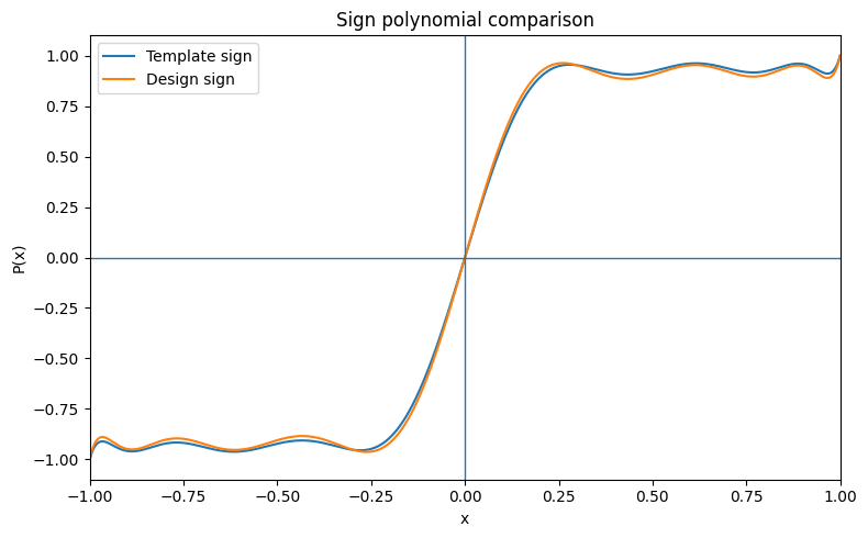
Output 1 (cell 8):
Sign template
  Degree [polynomial degree]:   13
  Parity [polynomial parity]:   odd
  Bounded [boolean]:  True
  Coeffs[:6]: [  0.         6.129262   0.       -50.716      0.       251.527514]

Sign design
  Degree [polynomial degree]:   13
  Parity [polynomial parity]:   odd
  Bounded [boolean]:  True
  Coeffs[:6]: [  0.         6.457019   0.       -57.235917   0.       292.840318]
Output 2 (cell 10):
Sign approximation errors on |x| >= gamma [dimensionless x]
  Template max error: 0.0934552831696136
  Design   max error: 0.1154179522161527
  Template RMS error: 0.06614683867917648
  Design   RMS error: 0.08075997225292844
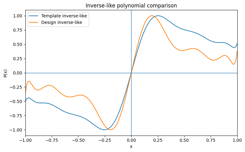
Output 3 (cell 12):
Inverse-like template
  Degree [polynomial degree]:   13
  Parity [polynomial parity]:   odd
  Bounded [boolean]:  True
  Coeffs[:6]: [  0.         6.728973   0.       -58.268765   0.       273.617565]

Inverse-like design
  Degree [polynomial degree]:   13
  Parity [polynomial parity]:   odd
  Bounded [boolean]:  True
  Coeffs[:6]: [   0.          8.358813    0.       -104.680547    0.        576.087771]
Output 4 (cell 14):
Inverse-like approximation errors against gamma/x on |x| >= gamma [dimensionless x]
  Template max error: 0.2880707591425103
  Design   max error: 0.16259666800719208
  Template rms error: 0.23148195494558868
  Design   rms error: 0.08536905981807905
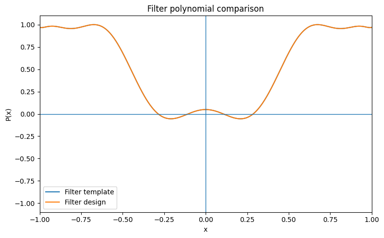
Output 5 (cell 16):
Filter template
  Degree [polynomial degree]:   12
  Parity [polynomial parity]:   even
  Bounded [boolean]:  True
  Coeffs[:6]: [ 0.048935  0.       -5.137833  0.       73.671274  0.      ]

Filter design
  Degree [polynomial degree]:   12
  Parity [polynomial parity]:   even
  Bounded [boolean]:  True
  Coeffs[:6]: [ 0.048935  0.       -5.137833  0.       73.671274  0.      ]
Output 6 (cell 18):
Filter approximation errors on [-1, 1] [dimensionless x]
  Template max error: 0.09099962265482087
  Design   max error: 0.09099962265482087
  Template rms error: 0.04297312621293089
  Design   rms error: 0.04297312621293089
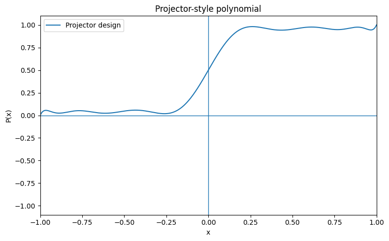
Output 7 (cell 20):
Projector design
  Degree [polynomial degree]:   13
  Parity [polynomial parity]:   mixed
  Bounded [boolean]:  True
  Coeffs[:6]: [  0.5        3.228509   0.       -28.617959   0.       146.420159]
Output 8 (cell 22):
Projector approximation errors on |x| >= gamma [dimensionless x]
  Max error: 0.05770897610807635
  RMS error: 0.04037998612646422
Output 9 (cell 24):
A = [[-0.9   0.    0.    0.    0.    0.    0.    0.  ]
 [ 0.   -0.55  0.    0.    0.    0.    0.    0.  ]
 [ 0.    0.   -0.3   0.    0.    0.    0.    0.  ]
 [ 0.    0.    0.   -0.1   0.    0.    0.    0.  ]
 [ 0.    0.    0.    0.    0.1   0.    0.    0.  ]
 [ 0.    0.    0.    0.    0.    0.3   0.    0.  ]
 [ 0.    0.    0.    0.    0.    0.    0.55  0.  ]
 [ 0.    0.    0.    0.    0.    0.    0.    0.9 ]]
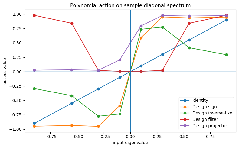
Output 10 (cell 25):
Diag entries:
[-0.9  -0.55 -0.3  -0.1   0.1   0.3   0.55  0.9 ]

Design sign on diag:
[-0.9488   -0.9341   -0.951784 -0.591317  0.591317  0.951784  0.9341
  0.9488  ]

Design inverse-like on diag:
[-0.293721 -0.41768  -0.774708 -0.736804  0.736804  0.774708  0.41768
  0.293721]

Design filter on diag:
[0.979311 0.841569 0.023234 0.004676 0.004676 0.023234 0.841569 0.979311]

Design projector on diag:
[0.0256   0.03295  0.024108 0.204342 0.795658 0.975892 0.96705  0.9744  ]
Output 11 (cell 27):
Diag(sign_design(A)) via spectral helper:
[-0.9488   -0.9341   -0.951784 -0.591317  0.591317  0.951784  0.9341
  0.9488  ]

Diag(filter_design(A)) via spectral helper:
[0.979311 0.841569 0.023234 0.004676 0.004676 0.023234 0.841569 0.979311]

Diag(projector_design(A)) via spectral helper:
[0.0256   0.03295  0.024108 0.204342 0.795658 0.975892 0.96705  0.9744  ]
Output 12 (cell 31):
Sign template
Degree [polynomial degree]: 13
Parity [polynomial parity]: odd
bounded [boolean]: True
max_abs_on_grid: 0.9999999999999876
Sign design
Degree [polynomial degree]: 13
Parity [polynomial parity]: odd
bounded [boolean]: True
max_abs_on_grid: 0.9999999999999538
Inverse template
Degree [polynomial degree]: 13
Parity [polynomial parity]: odd
bounded [boolean]: True
max_abs_on_grid: 1.0
Inverse design
Degree [polynomial degree]: 13
Parity [polynomial parity]: odd
bounded [boolean]: True
max_abs_on_grid: 1.0
Filter template
Degree [polynomial degree]: 12
Parity [polynomial parity]: even
bounded [boolean]: True
max_abs_on_grid: 0.9999996169147369
Filter design
Degree [polynomial degree]: 12
Parity [polynomial parity]: even
bounded [boolean]: True
max_abs_on_grid: 0.9999996169147369
Projector design
Degree [polynomial degree]: 13
Parity [polynomial parity]: mixed
bounded [boolean]: True
max_abs_on_grid: 0.9999999999999769
--- safe-region scalar checks ---
Sign template max err on |x| >= gamma [dimensionless x]: 0.0934552831696136
Sign design max err on |x| >= gamma [dimensionless x]: 0.1154179522161527
Inverse template max err vs gamma/x on |x| >= gamma [dimensionless x]: 0.2880707591425103
Inverse design max err vs gamma/x on |x| >= gamma [dimensionless x]: 0.16259666800719208
Filter template max err on [-1,1]: 0.09099962265482087
Filter design max err on [-1,1]: 0.09099962265482087
Projector design max err on |x| >= gamma [dimensionless x]: 0.05770897610807635
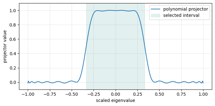
--- projector checkpoints ---
x=-0.80 -> value 0.048090
x=-0.50 -> value 0.047393
x=-0.25 -> value 0.019036
x=+0.25 -> value 0.980964
x=+0.50 -> value 0.952607
x=+0.80 -> value 0.951910
--- Diagonal outputs ---
Diag entries:
[-0.9 -0.55 -0.3 -0.1 0.1 0.3 0.55 0.9 ]
Design sign:
[-0.9488 -0.9341 -0.951784 -0.591317 0.591317 0.951784 0.9341
0.9488 ]
Design inverse-like:
[-0.293721 -0.41768 -0.774708 -0.736804 0.736804 0.774708 0.41768
0.293721]
Design filter:
[0.979311 0.841569 0.023234 0.004676 0.004676 0.023234 0.841569 0.979311]
Design projector:
[0.0256 0.03295 0.024108 0.204342 0.795658 0.975892 0.96705 0.9744 ]
--- Spectral consistency checks ---
Sign diag consistency [boolean]: True
Filter diag consistency [boolean]: True
Projector diag consistency [boolean]: True
Output 13 (cell 33):
Sign_design_max_error: 1.154e-01
Inverse_design_max_error: 1.626e-01
Projector_design_max_error: 5.771e-02
validation: passed
11_QSVT_Algorithm_Workflows.ipynb
Source: notebooks/tutorials/11_QSVT_Algorithm_Workflows.ipynb
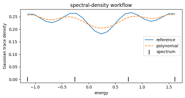
Output 1 (cell 4):
Eigenvalues: [-1.1405 -0.258 0.7399 1.6086]
Output 2 (cell 6):
Polynomial residual: 0.06293241692724773
Relative error: 0.04364138768069171
Output 3 (cell 8):
Ground state overlap [probability]: 9.855e-01
Ground filter state error: 1.252e-03
Hamiltonian state error: 3.953e-08
Resolvent response error: 1.695e-01
Spectral density error: 4.670e-02
Thermal density error: 6.412e-08
Output 4 (cell 12):
thermal-gibbs-workflow
report keys [count/list]: ['beta', 'coeffs', 'degree', 'density_matrix_relative_error', 'implementation_kind', 'mode', 'operator_relative_error', 'polynomial_boltzmann_operator'] ...
12_QSVT_Reports_CLI_and_Artifacts.ipynb
Source: notebooks/tutorials/12_QSVT_Reports_CLI_and_Artifacts.ipynb
Output 1 (cell 4):
design-workflow sign design_sign_polynomial
Degree [polynomial degree]: 9
Max error: 0.24846221549762104
Bounded margin: -8.881784197001252e-15
Output 2 (cell 6):
JSON exists [boolean]: True
Plot exists [boolean]: True
Loaded mode [string]: design-workflow
Loaded coeff count [count]: 10
Output 3 (cell 8):
CLI design-workflow summary
---------------------------
Mode [string]           : design-workflow
Report written [path] : True
Plot written [path]   : False
Output path [path]    : cli-sign-workflow.json
Report kind [string]    : sign
Coefficients [count]   : 10
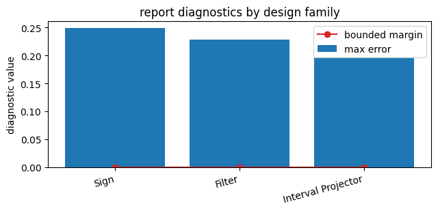
Output 4 (cell 10):
Sign max_error=2.485e-01, margin=-8.882e-15, parity [polynomial parity]=odd
Filter max_error=2.284e-01, margin=-1.998e-15, parity [polynomial parity]=even
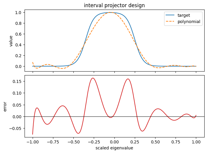
Interval Projector max_error=1.968e-01, margin=0.000e+00, parity [polynomial parity]=mixed
13_QSVT_Design_Tradeoffs.ipynb
Source: notebooks/tutorials/13_QSVT_Design_Tradeoffs.ipynb
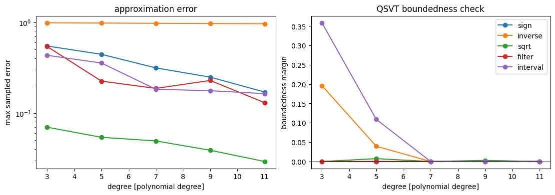
Output 1 (cell 4):
Representative degree-3 designs
-------------------------------
Family   : sign | inverse | sqrt | filter | interval
Degree : 3 | 3 | 3 | 3 | 3
Max error : 0.5479 | 0.9892 | 0.06978 | 0.5407 | 0.4328
Bounded margin : 0 | 0.1963 | 0 | 0 | 0.3587
Parity : odd | odd | mixed | even | mixed
Bounded : True | True | True | True | True
Output 2 (cell 6):
<matplotlib.legend.Legend at 0x745223280ec0>
Output 3 (cell 8):
Max error: 0.1632978061045941
Bounded margin: 1.1102230246251565e-16
14_QSVT_Resource_Proxy_Limits.ipynb
Source: notebooks/tutorials/14_QSVT_Resource_Proxy_Limits.ipynb
Output 1 (cell 4):
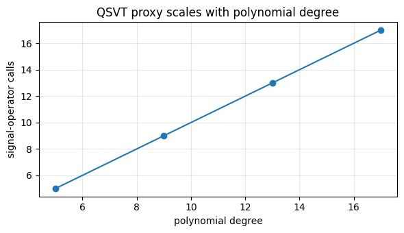
Degree [polynomial degree]= 5 , Signal_calls [operator calls]= 5 , Encoding_qubits [qubits]= 4
Degree [polynomial degree]= 9 , Signal_calls [operator calls]= 9 , Encoding_qubits [qubits]= 4
Degree [polynomial degree]= 13 , Signal_calls [operator calls]= 13 , Encoding_qubits [qubits]= 4
Degree [polynomial degree]= 17 , Signal_calls [operator calls]= 17 , Encoding_qubits [qubits]= 4
Output 2 (cell 7):
Exact rank [states]: 2
Rank proxy [states]: 1.955
Leakage: 0.017
State weight error: 0.008
15_Block_Encoded_QSVT_Workflow.ipynb
Source: notebooks/tutorials/15_Block_Encoded_QSVT_Workflow.ipynb
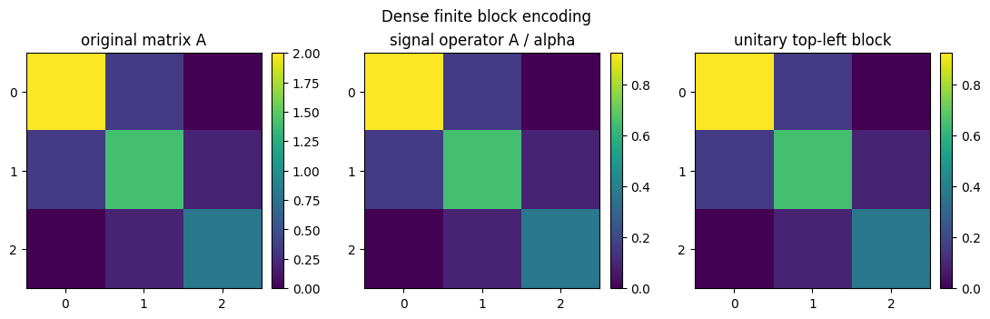
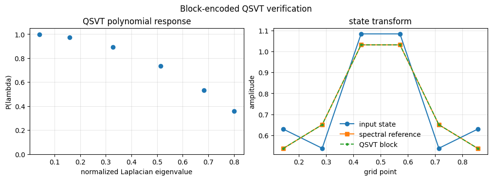
Output 1 (cell 4):
alpha: 2.166226041207235
logical_dimension: 3
unitary_dimension: 6
block_error: 0.0
unitarity_error: 1.275387486109542e-15
reconstruction_error: 0.0
Output 2 (cell 7):
workflow: block-encoded-qsvt-workflow
pennylane_qsvt_check: succeeded
operator_relative_error: 1.000085679496161e-12
state_relative_error: 1.0000638768158241e-12
Output 3 (cell 9):
execution_kind: pennylane-qnode-statevector-qsvt-execution
gate_types: {'StatePrep': 1, 'QSVT': 1}
logical_success_probability: 0.967454109399
qnode_real_error: 9.771e-13
qnode_max_imag: 5.830e-02
Output 4 (cell 12):
validation: passed
16_Sparse_Oracle_Assumptions.ipynb
Source: notebooks/tutorials/16_Sparse_Oracle_Assumptions.ipynb
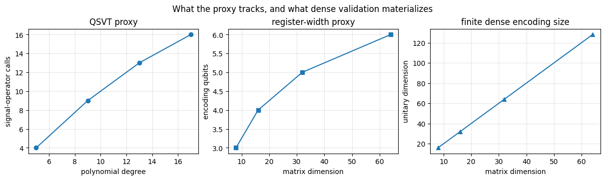
Output 1 (cell 4):
model                          implemented_here  visible_cost                           omitted_cost
-----------------------------  ----------------  -------------------------------------  -----------------------------------------
dense finite matrix            yes               matrix dimension and dense validation  scalable data loading
explicit dense block encoding  finite only       unitary dimension and block error      asymptotic oracle construction
sparse-access block encoding   no                degree and signal-call proxy only      row oracle, value oracle, normalization
end-to-end quantum workflow    no                not estimated                          state preparation, readout, amplification
Output 2 (cell 6):
dimension= 8 degree= 4 signal_calls= 4 encoding_qubits= 3
dimension= 16 degree= 9 signal_calls= 9 encoding_qubits= 4
dimension= 32 degree= 13 signal_calls= 13 encoding_qubits= 5
dimension= 64 degree= 16 signal_calls= 16 encoding_qubits= 6
Output 3 (cell 9):
implementation_kind: polynomial-resource-proxy
truth_status: proxy_only
requires_block_encoding: True
requires_state_preparation: True
omitted_costs:
 - block_encoding_construction
 - state_preparation
 - amplitude_amplification
 - error_correction
 - hardware_compilation
Output 4 (cell 11):
validation: passed
17_QSVT_Compatibility_Failure_Cases.ipynb
Source: notebooks/tutorials/17_QSVT_Compatibility_Failure_Cases.ipynb
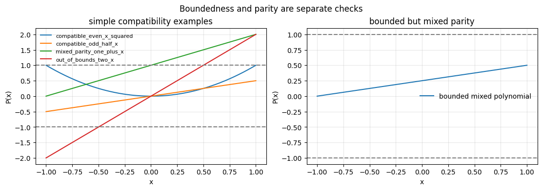
Output 1 (cell 4):
candidate                         degree  parity  bounded  compatible  reasons
----------------------------------------------------------------------------------------
compatible_even_x_squared       2       even    True     True        none
compatible_odd_half_x           1       odd     True     True        none
mixed_parity_one_plus_x         1       mixed   False    False       mixed_parity, out_of_bounds
out_of_bounds_two_x             1       odd     False    False       out_of_bounds
bounded_mixed_offset_slope      1       mixed   True     False       mixed_parity
Output 2 (cell 7):
compatible_even_x_squared: max_abs=1.000, parity=even, compatible=True, reasons=[]
compatible_odd_half_x: max_abs=0.500, parity=odd, compatible=True, reasons=[]
mixed_parity_one_plus_x: max_abs=2.000, parity=mixed, compatible=False, reasons=['mixed_parity', 'out_of_bounds']
out_of_bounds_two_x: max_abs=2.000, parity=odd, compatible=False, reasons=['out_of_bounds']
bounded_mixed_offset_slope: max_abs=0.500, parity=mixed, compatible=False, reasons=['mixed_parity']
Output 3 (cell 9):
validation: passed
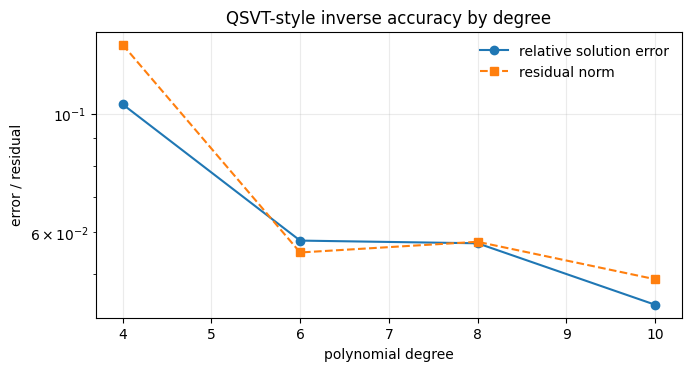
18_QSVT_Linear_System_Comparisons.ipynb
Source: notebooks/tutorials/18_QSVT_Linear_System_Comparisons.ipynb
Output 1 (cell 4):
solver                         implementation_kind                 degree  iterations  residual_norm  relative_solution_error
-----------------------------  ----------------------------------  ------  ----------  -------------  -----------------------
dense_solve                    classical-dense-reference           8       -           5.551e-17      0.000e+00
conjugate_gradient             classical-iterative-reference       8       2           5.551e-17      0.000e+00
qsvt_style_polynomial_inverse  dense-spectral-polynomial-workflow  8       -           0.0575533      0.0571796
Output 2 (cell 6):
quantity                   value
-------------------------  ---------
degree                     8
gamma                      0.565741
condition_number_2         1.76759
gamma_condition_proxy      1.76759
polynomial_relative_error  0.0571796
Output 3 (cell 7):
degree  relative_solution_error  residual_norm
------  -----------------------  -------------
4       0.104276                 0.134979
6       0.0578489                0.0549513
8       0.0571796                0.0575533
10      0.0438395                0.0489511
19_HHL_Linear_System_Solver.ipynb
Source: notebooks/tutorials/19_HHL_Linear_System_Solver.ipynb
Output 1 (cell 8):
A =
[[ 1.25     -0.433013]
 [-0.433013  1.75    ]]

normalized |b> = [0.894427 0.447214]
eigenvalues = [1. 2.]
phase indices = [1 2]
estimated eigenvalues = [1. 2.]
rotation amplitudes C / lambda = [1.  0.5]
success probability = 0.9973076211353317
HHL state = [0.880635 0.473796]
dense solution state = [0.880635 0.473796]
state error = 1.5700924586837752e-16
fidelity = 0.9999999999999998
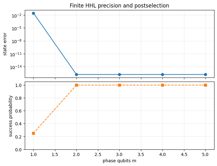
Output 2 (cell 10):
m  grid_size  phase_indices  success_probability  state_error  fidelity
-  ---------  -------------  -------------------  -----------  --------
1  2          (1, 1)         0.25                 0.0299475    0.999103
2  4          (1, 2)         0.997308             1.570e-16    1
3  8          (2, 4)         0.997308             1.570e-16    1
4  16         (4, 8)         0.997308             1.570e-16    1
5  32         (8, 16)        0.997308             1.570e-16    1
Output 3 (cell 13):
A_sweep eigenvalues = [1. 1.414214]
normalized |b_sweep> = [0.707107+0.j 0.707107+0.j]
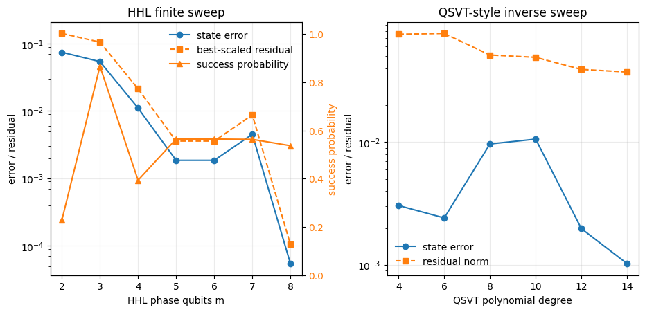
m phase_indices estimated_eigenvalues state_error best_scaled_residual_norm success_probability
- ------------- --------------------- ----------- ------------------------- -------------------
2 (1, 1) (1.570796, 1.570796) 0.074533 0.141775 0.227973
3 (1, 2) (0.785398, 1.570796) 0.054061 0.105332 0.866077
4 (3, 4) (1.178097, 1.570796) 0.0110711 0.0213574 0.393407
5 (5, 7) (0.981748, 1.374447) 0.00185627 0.00358702 0.564462
6 (10, 14) (0.981748, 1.374447) 0.00185627 0.00358702 0.564462
7 (20, 29) (0.981748, 1.423534) 0.00451793 0.00874009 0.56311
8 (41, 58) (1.006291, 1.423534) 5.438e-05 1.051e-04 0.536872
Output 4 (cell 15):
method              implementation_kind                 state_error  success_probability  residual_norm  relative_vector_error  phase_qubits  degree  gamma
------------------  ----------------------------------  -----------  -------------------  -------------  ---------------------  ------------  ------  --------
HHL finite          finite-spectral-hhl-simulation      5.438e-05    0.536872             1.051e-04      -                      8             -       -
QSVT-style inverse  dense-spectral-polynomial-workflow  0.00966862   -                    0.0512108      0.0367455              -             8       0.707107

QSVT-style solver rows:
solver                         implementation_kind                 degree  residual_norm  relative_solution_error
-----------------------------  ----------------------------------  ------  -------------  -----------------------
dense_solve                    classical-dense-reference           8       0.000e+00      0.000e+00
qsvt_style_polynomial_inverse  dense-spectral-polynomial-workflow  8       0.0512108      0.0367455
Output 5 (cell 17):
HHL non-exact phase-estimation sweep:
m  state_error  best_scaled_residual_norm  success_probability
-  -----------  -------------------------  -------------------
2  0.074533     0.141775                   0.227973
3  0.054061     0.105332                   0.866077
4  0.0110711    0.0213574                  0.393407
5  0.00185627   0.00358702                 0.564462
6  0.00185627   0.00358702                 0.564462
7  0.00451793   0.00874009                 0.56311
8  5.438e-05    1.051e-04                  0.536872

QSVT-style degree sweep:
degree  state_error  residual_norm  relative_vector_error
------  -----------  -------------  ---------------------
4       0.00304798   0.0756114      0.052888
6       0.00241537   0.0767715      0.0538402
8       0.00966862   0.0512108      0.0367455
10      0.0105851    0.049006       0.0350409
12      0.00197623   0.0390797      0.0279143
14      0.00102514   0.0372169      0.0264762