Real-Example Results
This generated page displays embedded setup schematics, diagnostic plots, and text outputs from every real-example notebook.
Current Status
Source notebooks:
notebooks/real_examples/Notebooks displayed:
30Embedded plot artefacts displayed:
55Plain-text notebook results displayed:
80Plot manifest:
results/tables/real_examples_plot_manifest.csv
Regeneration
Execute notebooks, extract their embedded outputs, and refresh this page with:
python scripts/extract_notebook_plots.py --preset real-examples --execute --write-docs
Notebook Results
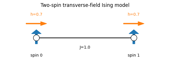
01_ground_state_filtering.ipynb
Source: notebooks/real_examples/01_ground_state_filtering.ipynb
Output 1 (cell 6):
Energies [model energy units]: [-1.7205 -1. 1. 1.7205]
Output 2 (cell 10):
Cutoff [model energy units]: -1.3602325267042625
Scale: 3.0806975801127883
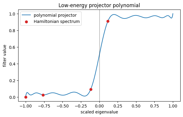
Scaled Energies [model energy units]: [-1. -0.7661 -0.1169 0.1169]
Output 3 (cell 12):
Projector Error: 0.13103683490762716
Idempotence Error: 0.11947057773046423
Output 4 (cell 14):
Initial Ground Overlap [probability]: 0.21077170866211486
Filtered Ground Overlap [probability]: 0.9974954270617575
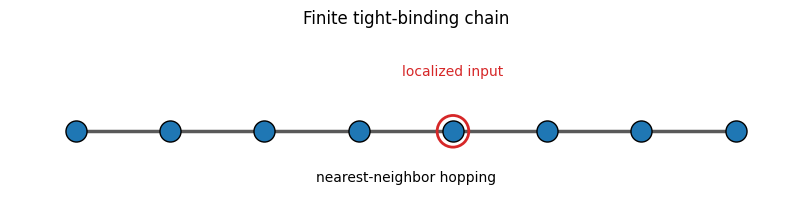
02_tight_binding_band_filter.ipynb
Source: notebooks/real_examples/02_tight_binding_band_filter.ipynb
Output 1 (cell 6):
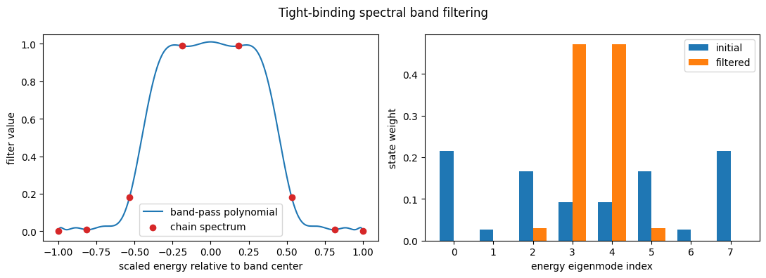
Energies [hopping units]: [-1.8794 -1.5321 -1. -0.3473 0.3473 1. 1.5321 1.8794]
Output 2 (cell 10):
Band Weights [probability]: [-0. 0.0083 0.1822 0.9885 0.9885 0.1822 0.0083 -0. ]
03_imaginary_time_filtering.ipynb
Source: notebooks/real_examples/03_imaginary_time_filtering.ipynb
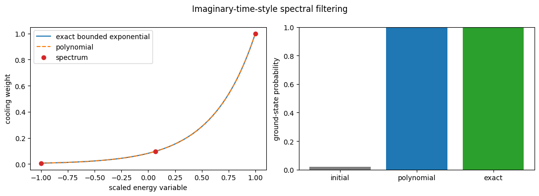
Output 1 (cell 6):
Energies [model energy units]: [0.2 0.8193 1.5306]
Output 2 (cell 8):
Scaled Energies [scaled model energy units]: [-1. 0.0691 1. ]
Output 3 (cell 10):
Operator Error: 1.852552687200035e-11
Output 4 (cell 12):
Initial Ground Weight [probability]: 0.018745945993631295
Cooled Ground Weight [probability]: 0.9930808704605139
Exact Ground Weight [probability]: 0.9930808704691421
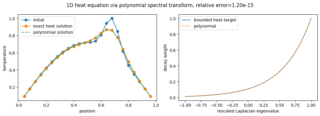
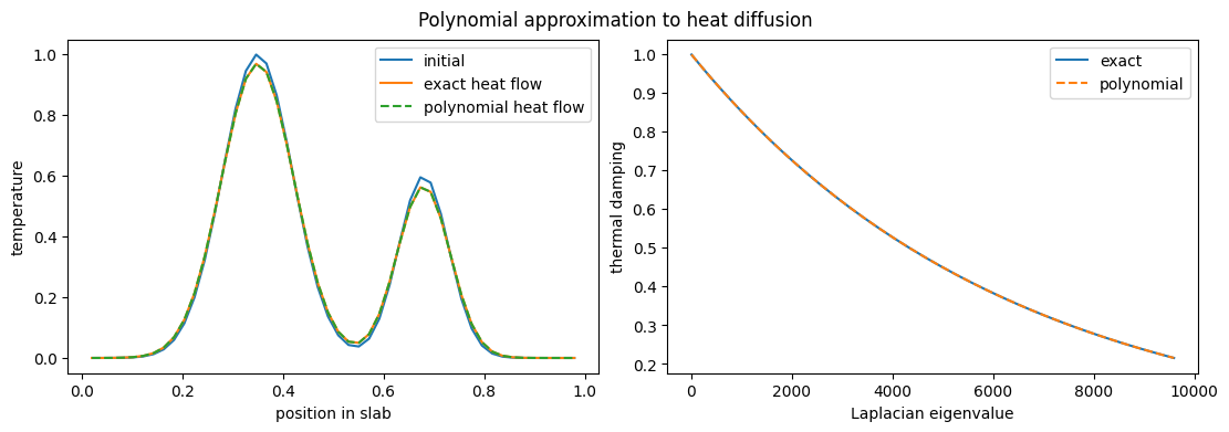
04_heat_equation_pde.ipynb
Source: notebooks/real_examples/04_heat_equation_pde.ipynb
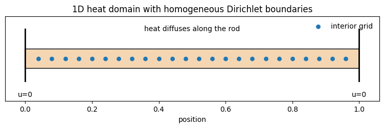
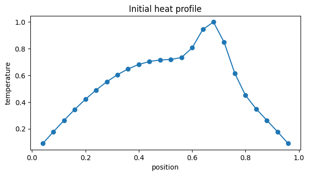
Output 1 (cell 6):
First 5 Eigenvalues [inverse grid-length units]: [  9.8566  39.271   87.7794 154.6166 238.7288]
Last Eigenvalue [inverse grid-length units]: 2490.1433766430973
Output 2 (cell 12):
First Eigenvalue [model spectral units]: -0.9999999999999999
Last Eigenvalue [model spectral units]: 1.0000000000000002
Beta: 2.232258077957575
Prefactor: 0.9824145391823961
Output 3 (cell 14):
Relative Error: 1.2039058554241987e-15
05_poisson_equation_pde.ipynb
Source: notebooks/real_examples/05_poisson_equation_pde.ipynb
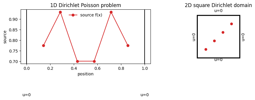
Output 1 (cell 6):
First Eigenvalue [inverse grid-length units]: 9.705050945562935
Last Eigenvalue [inverse grid-length units]: 186.29494905443704
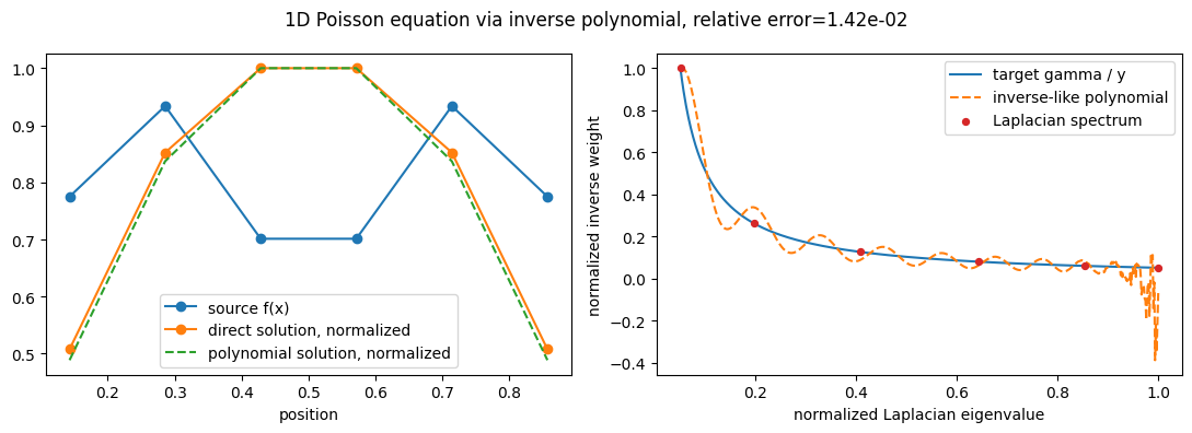
Output 2 (cell 10):
Gamma: 0.05209508360168709
Condition Number: 19.1956693580892
Output 3 (cell 12):
Relative Error: 0.014150625457763643
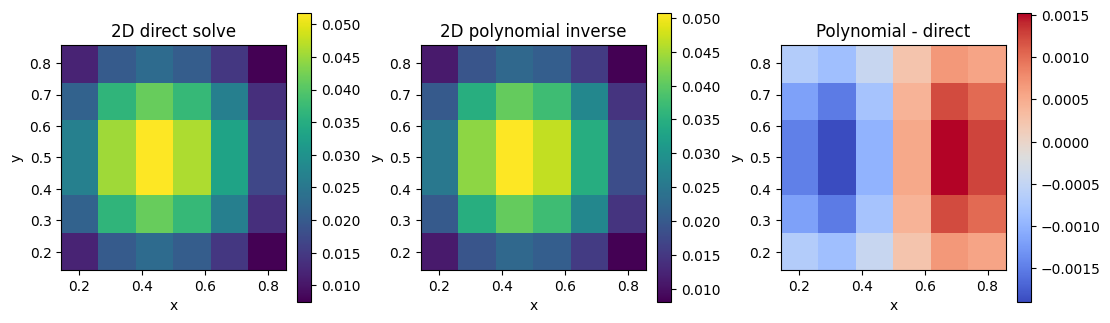
Output 4 (cell 15):
Gamma: 0.05209508360168687
Condition Number: 19.195669358089283
Matrix Shape [rows, cols]: (36, 36)
Output 5 (cell 17):
Relative Error: 0.034962641317254864
Output 6 (cell 21):
1D condition_number: 19.196
1D relative_error: 1.415e-02
2D condition_number: 19.196
2D relative_error: 3.496e-02
validation: passed
06_hamiltonian_simulation_schrodinger_dynamics.ipynb
Source: notebooks/real_examples/06_hamiltonian_simulation_schrodinger_dynamics.ipynb
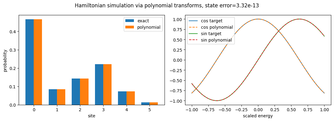
Output 1 (cell 5):
State Error: 3.324978121461713e-13
07_quantum_chemistry_h2_toy_solver.ipynb
Source: notebooks/real_examples/07_quantum_chemistry_h2_toy_solver.ipynb
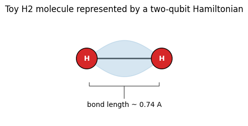
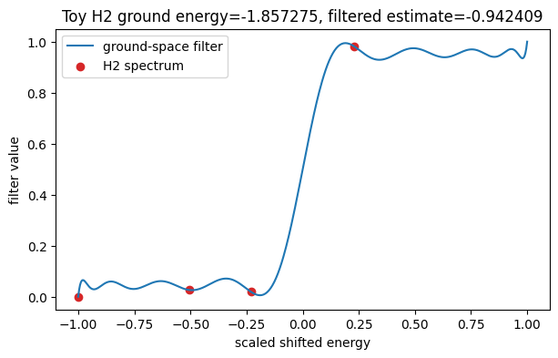
Output 1 (cell 4):
Ground Energy [hartree]: -1.85727503020238
Output 2 (cell 7):
Initial Overlap [probability]: 3.4911941432755493e-35
Filtered Overlap [probability]: 6.719832005838039e-33
Energy Estimate [hartree]: -0.9424088608987823
08_greens_function_response.ipynb
Source: notebooks/real_examples/08_greens_function_response.ipynb
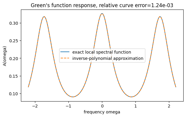
Output 1 (cell 4):
Response Error: 0.001236443161688136
09_spectral_density_estimation.ipynb
Source: notebooks/real_examples/09_spectral_density_estimation.ipynb
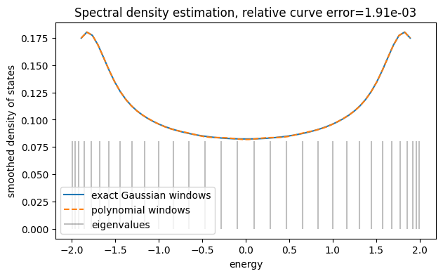
Output 1 (cell 4):
Curve Error: 0.0019122824182919095
10_gibbs_state_thermal_weights.ipynb
Source: notebooks/real_examples/10_gibbs_state_thermal_weights.ipynb
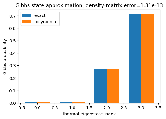
Output 1 (cell 4):
Rho Error: 1.8102065129092896e-13
11_transport_physics_landauer_chain.ipynb
Source: notebooks/real_examples/11_transport_physics_landauer_chain.ipynb
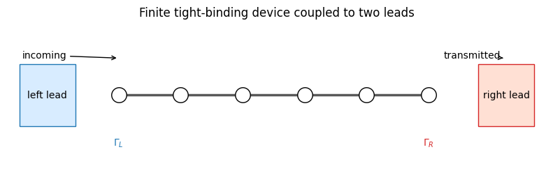
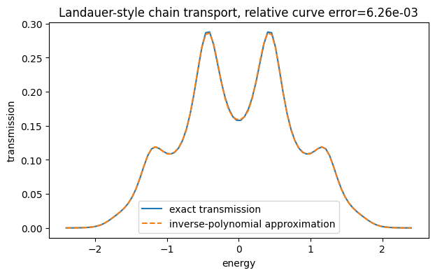
Output 1 (cell 4):
Curve Error: 0.00625639231073604
12_tensor_network_hybrid_filtering.ipynb
Source: notebooks/real_examples/12_tensor_network_hybrid_filtering.ipynb
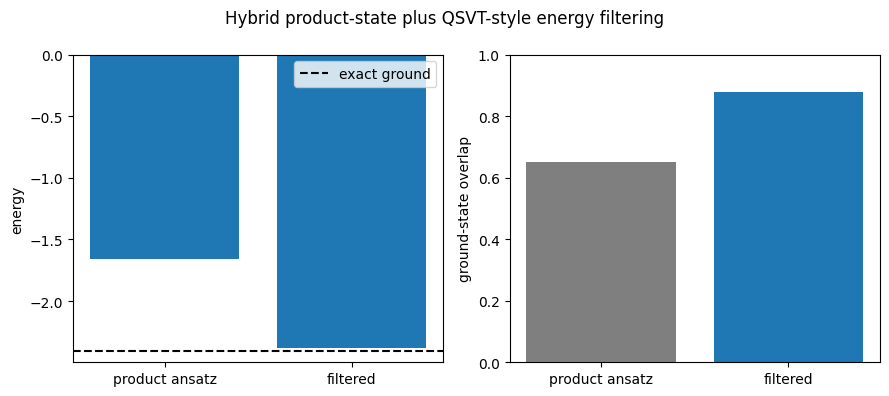
Output 1 (cell 4):
Initial Energy [model energy units]: -1.6606649134095948
Filtered Energy [model energy units]: -2.3777913739261485
Initial Overlap [probability]: 0.651393401185215
Filtered Overlap [probability]: 0.8772155174329324
13_heat_equation_2d_pde.ipynb
Source: notebooks/real_examples/13_heat_equation_2d_pde.ipynb
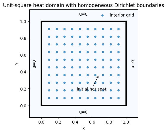
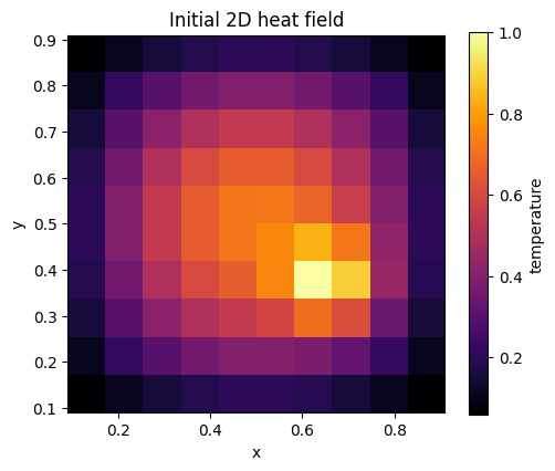
Output 1 (cell 6):
First 5 Eigenvalues [inverse grid-length units]: [19.6054 48.2193 48.2193 76.8333 93.3264]
Last Eigenvalue [inverse grid-length units]: 948.3945992294168
Matrix Shape [rows, cols]: (100, 100)
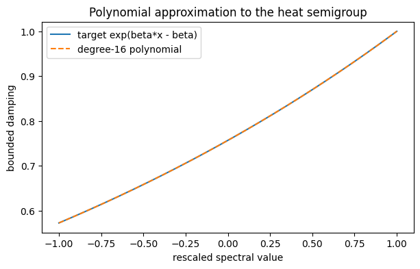
Output 2 (cell 12):
First Eigenvalue [model spectral units]: -1.0000000000000009
Last Eigenvalue [model spectral units]: 1.000000000000001
Beta: 0.27863675953765005
Prefactor: 0.9883056759592374
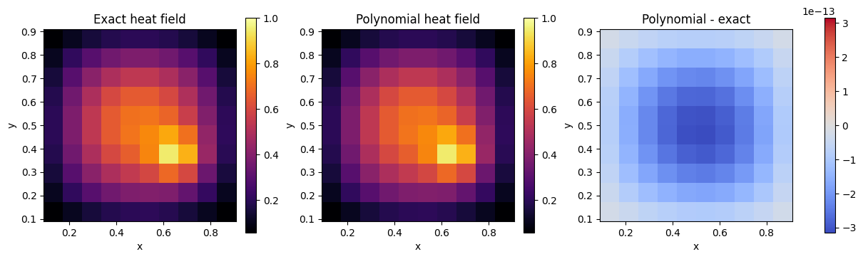
Output 3 (cell 14):
Relative Error: 4.054746215837559e-13
Output 4 (cell 18):
Maximum Approximation Error: 4.127809205556332e-13
Output 5 (cell 20):
relative_error: 4.055e-13
max_abs_difference [field units]: 3.149e-13
validation: passed
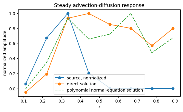
14_advection_diffusion_pde.ipynb
Source: notebooks/real_examples/14_advection_diffusion_pde.ipynb
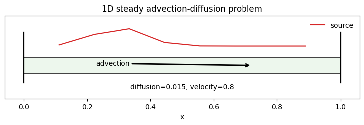
Output 1 (cell 5):
Non-normality [operator-norm units]: 24.743080487279663
Output 2 (cell 9):
Gamma: 0.057449326656195406
1.0 / Gamma: 17.406644397844456
Relative Error: 0.22813071877482616
Output 3 (cell 12):
non_normality [operator-norm units]: 2.474e+01
normal_equation_condition_number: 17.407
relative_error: 2.281e-01
validation: passed
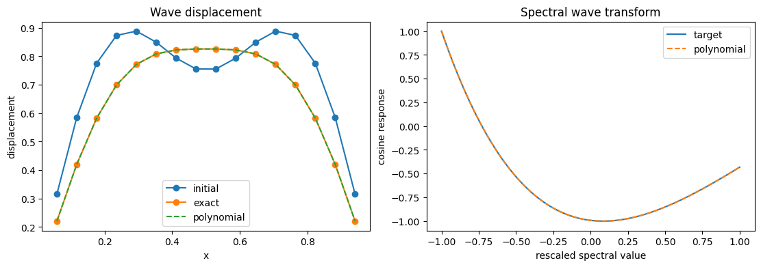
15_wave_equation_dynamics.ipynb
Source: notebooks/real_examples/15_wave_equation_dynamics.ipynb
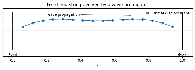
Output 1 (cell 5):
First Eigenvalue [model spectral units]: -0.9828268973302636
Last Eigenvalue [model spectral units]: 0.9999999999999998
Beta: 4.265725211247927
Output 2 (cell 9):
Relative Error: 2.942102758155022e-15
Output 3 (cell 12):
beta: 4.266
relative_error: 2.942e-15
validation: passed
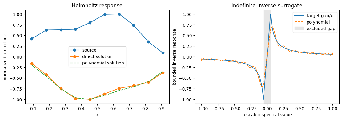
16_helmholtz_equation_pde.ipynb
Source: notebooks/real_examples/16_helmholtz_equation_pde.ipynb
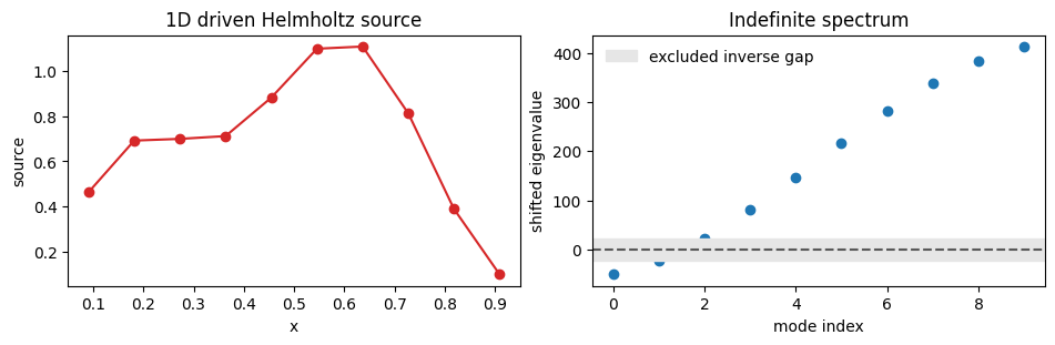
Output 1 (cell 5):
First 4 Eigenvalues [inverse grid-length units]: [-51.1675 -22.5535  22.5535  80.4994]
Last Eigenvalue [inverse grid-length units]: 413.22712589466073
Gap [model energy units]: 0.05457901297346752
Output 2 (cell 9):
Relative Error: 0.16873834910647584
Maximum Fit Error: 0.3658574904383274
Output 3 (cell 12):
spectral_gap [model energy units]: 5.458e-02
max_fit_error: 3.659e-01
relative_error: 1.687e-01
validation: passed
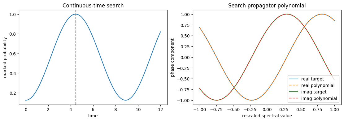
17_quantum_walk_search_toy.ipynb
Source: notebooks/real_examples/17_quantum_walk_search_toy.ipynb
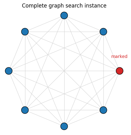
Output 1 (cell 5):
Eigenvalues [oracle energy units]: [-1.2286 -0.5214  0.125   0.125   0.125   0.125   0.125   0.125 ]
Eigenvalues of A: [-1.  1.]
Output 2 (cell 9):
Best Time [inverse energy units]: 4.452830188679245
Best Probability [probability]: 0.9999891776297675
Output 3 (cell 11):
State Error: 1.0120998885188465e-13
Polynomial Probability [probability]: 0.9999891776298157
Output 4 (cell 14):
best_time [inverse energy units]: 4.453
best_probability [probability]: 0.999989
poly_probability [probability]: 0.999989
state_error: 1.012e-13
validation: passed
18_ssh_chain_edge_state_filtering.ipynb
Source: notebooks/real_examples/18_ssh_chain_edge_state_filtering.ipynb
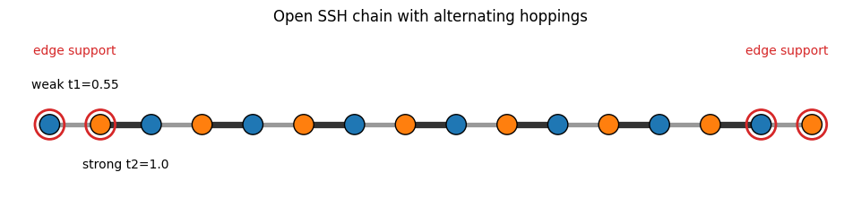
Output 1 (cell 6):
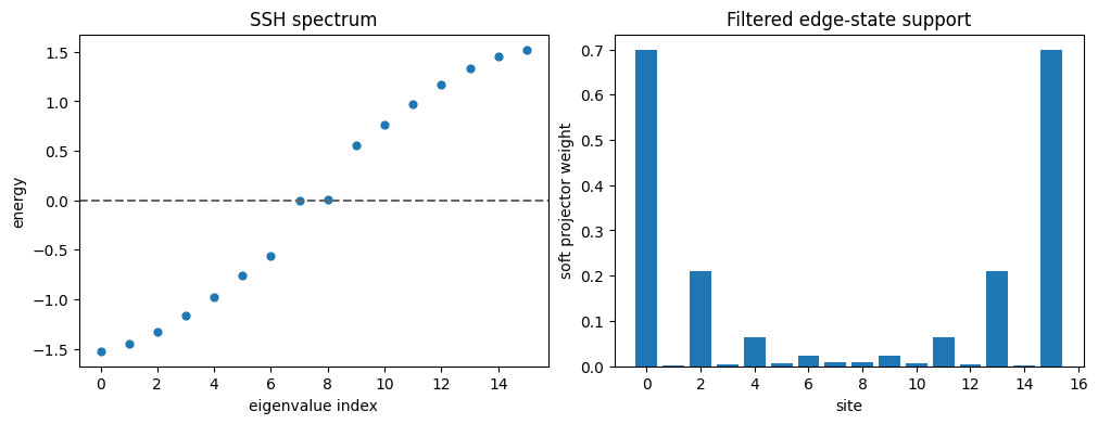
Near-Zero Eigenvalues [hopping units]: [-0.5577 -0.0058 0.0058 0.5577]
Output 2 (cell 10):
Edge Weight Fraction [probability]: 0.6880404379008599
Trace of Soft Edge Projector [states]: 2.0327822807342835
Output 3 (cell 13):
near_zero_eigenvalues [hopping units]: [-0.55766 -0.00584  0.00584  0.55766]
edge_weight_fraction [probability]: 0.688
projector_trace [states]: 2.033
validation: passed
19_anderson_localization.ipynb
Source: notebooks/real_examples/19_anderson_localization.ipynb
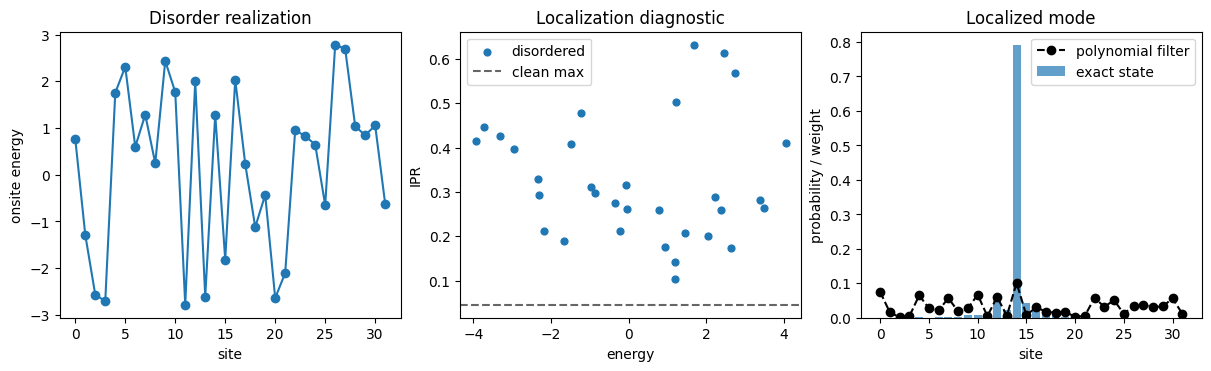
Output 1 (cell 5):
Localized IPR: 0.6321472059662562
Maximum Clean IPR: 0.045454545454545796
Output 2 (cell 7):
Peak Site [site index]: 14
Filtered Weight at Peak Site [probability]: 0.10072442254521352
Output 3 (cell 10):
localized_energy [hopping units]: 1.6901
localized_ipr: 0.6321
clean_max_ipr: 0.0455
peak_site_filter_weight [probability]: 0.1007
validation: passed
20_schrodinger_bound_states.ipynb
Source: notebooks/real_examples/20_schrodinger_bound_states.ipynb
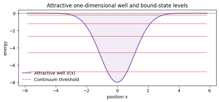
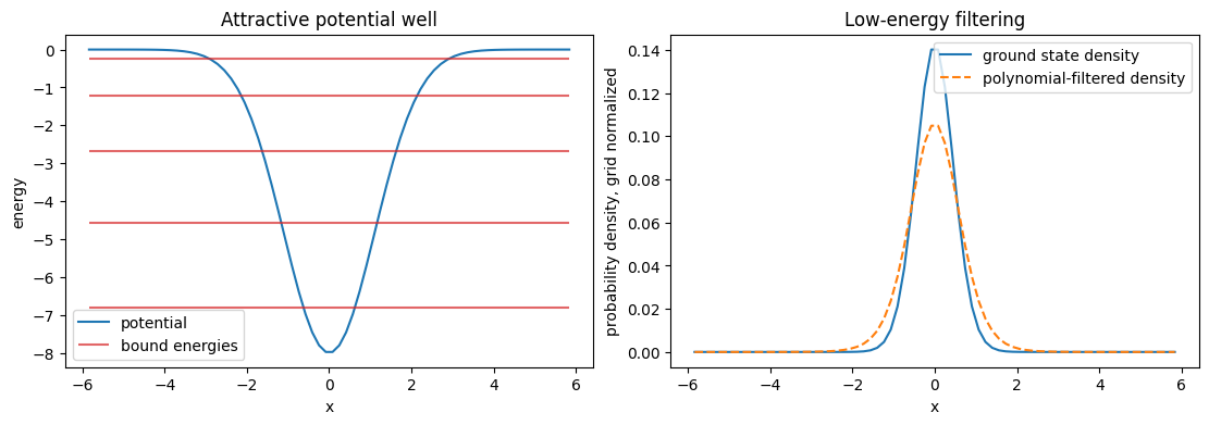
Output 1 (cell 5):
Eigenvalues [model energy units]: [-6.7968 -4.5635 -2.6903 -1.2181 -0.2361  0.1906]
Number of Bound States [states]: 5
Output 2 (cell 9):
Ground State Overlap [probability]: 0.9505375069652005
Filtered Energy [model energy units]: -6.586964339925885
Output 3 (cell 12):
lowest_energies [model energy units]: [-6.7968 -4.5635 -2.6903 -1.2181 -0.2361  0.1906]
n_bound [states]: 5
ground_overlap [probability]: 0.9505
filtered_energy [model energy units]: -6.5870
validation: passed
21_quantum_harmonic_oscillator_grid.ipynb
Source: notebooks/real_examples/21_quantum_harmonic_oscillator_grid.ipynb
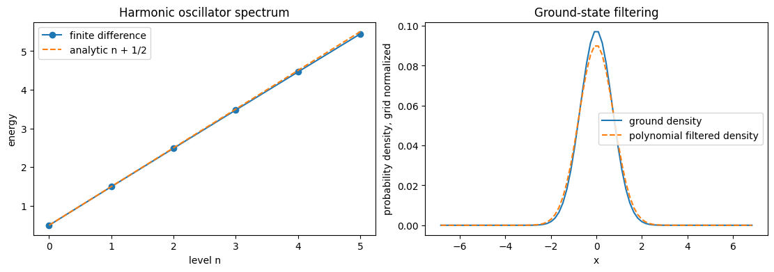
Output 1 (cell 5):
Eigenvalues [model energy units]: [0.4991 1.4953 2.4878 3.4765 4.4614 5.4424]
Spectrum Error [model energy units]: 0.02350013331927281
Output 2 (cell 6):
Ground State Overlap [probability]: 0.9969945579767748
Output 3 (cell 9):
finite_difference_energies [model energy units]: [0.4991 1.4953 2.4878 3.4765 4.4614 5.4424]
analytic_energies [model energy units]: [0.5 1.5 2.5 3.5 4.5 5.5]
spectrum_error_first_four [model energy units]: 2.3500e-02
ground_overlap [probability]: 0.9970
validation: passed
22_electrostatic_green_function_poisson.ipynb
Source: notebooks/real_examples/22_electrostatic_green_function_poisson.ipynb
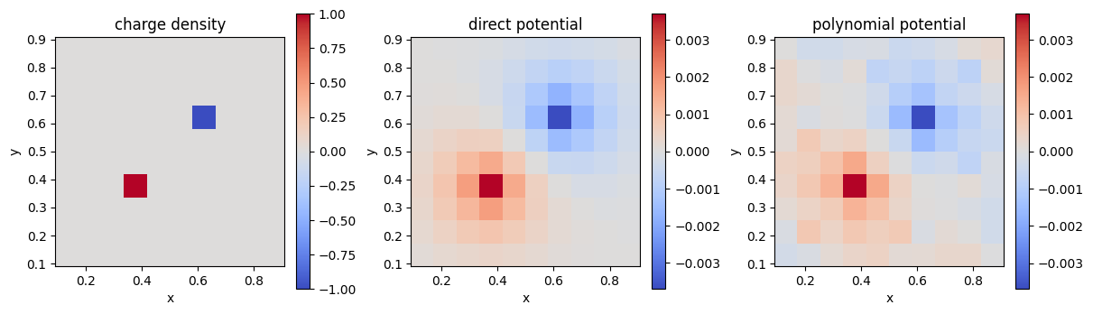
Output 1 (cell 5):
Potential at Positive Charge [potential units]: 0.0037023041787180174
Potential at Negative Charge [potential units]: -0.0037023041787180165
Sum of Charges [charge units]: 0.0
Output 2 (cell 7):
Relative Error: 0.2679780308568579
Selected Degree [polynomial degree]: 29
Condition Number: 48.37415007870855
Output 3 (cell 10):
condition_number: 48.374
positive_charge_potential [potential units]: 3.7023e-03
negative_charge_potential [potential units]: -3.7023e-03
selected_degree [polynomial degree]: 29
relative_error: 2.680e-01
validation: passed
23_coupled_oscillator_normal_modes.ipynb
Source: notebooks/real_examples/23_coupled_oscillator_normal_modes.ipynb
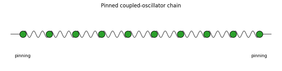
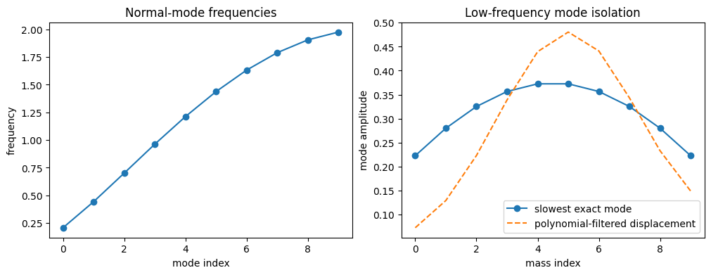
Output 1 (cell 5):
Frequencies [angular frequency units]: [0.2072 0.4426 0.7012 0.9629 1.2121]
Output 2 (cell 9):
Slow Mode Overlap [probability]: 0.9147264843650682
Output 3 (cell 12):
frequencies [angular frequency units]: [0.2072 0.4426 0.7012 0.9629 1.2121]
lowest_stiffness [angular frequency squared units]: 4.2916e-02
slow_mode_overlap [probability]: 0.9147
validation: passed
24_ising_phase_transition_filtering.ipynb
Source: notebooks/real_examples/24_ising_phase_transition_filtering.ipynb
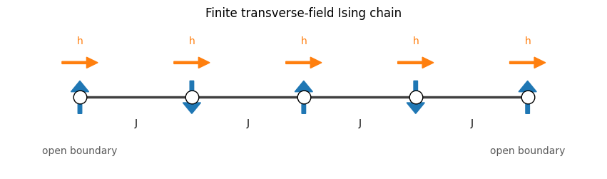
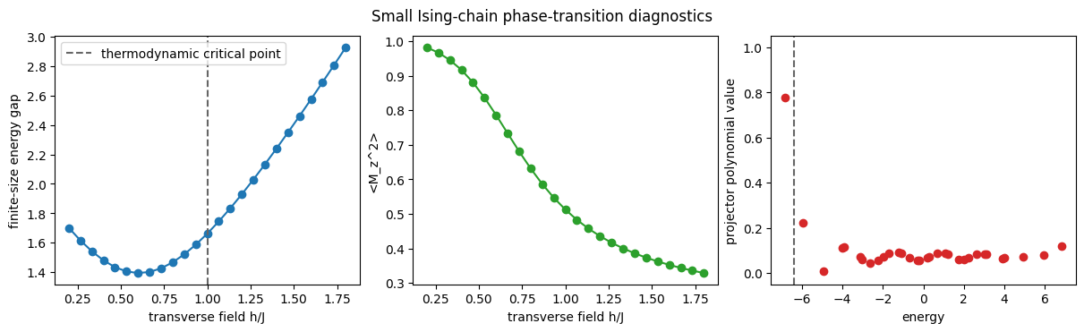
Output 1 (cell 5):
Ising sweep diagnostics
-----------------------
Minimum gap field [coupling ratio h/J]       : 0.6
Minimum gap [coupling units]             : 1.394
Maximum magnetization field [coupling ratio h/J] : 0.2
Maximum magnetization [magnetization squared]       : 0.9818
Output 2 (cell 9):
Projector eigenweights [probability]: [0.7761 0.2239 0.0087 0.1109 0.1143]
Projector error: 0.5286773050862152
Output 3 (cell 11):
minimum_doublet_gap_field [coupling ratio h/J]: 0.600
magnetization_drop [magnetization squared]: 0.653
projector_error: 0.529
validation: passed
25_diffusion_heat_treatment_slab.ipynb
Source: notebooks/real_examples/25_diffusion_heat_treatment_slab.ipynb
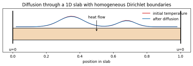
Output 1 (cell 5):
Relative Error: 2.8910082648989737e-15
Output 2 (cell 9):
relative_temperature_error: 0.0000
initial_norm [temperature units]: 2.7653
cooled_norm [temperature units]: 2.7152
validation: passed
26_graphene_nanoribbon_density_of_states.ipynb
Source: notebooks/real_examples/26_graphene_nanoribbon_density_of_states.ipynb
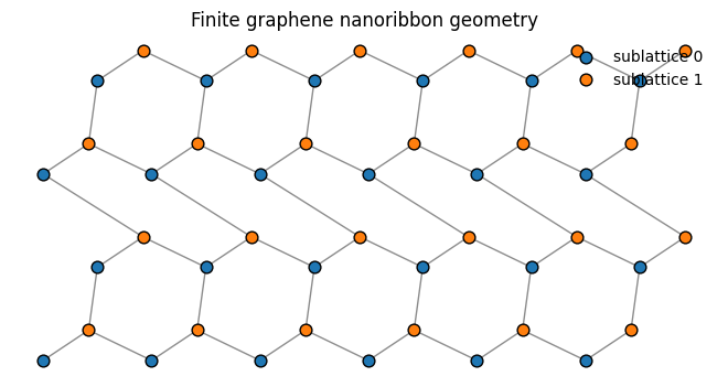
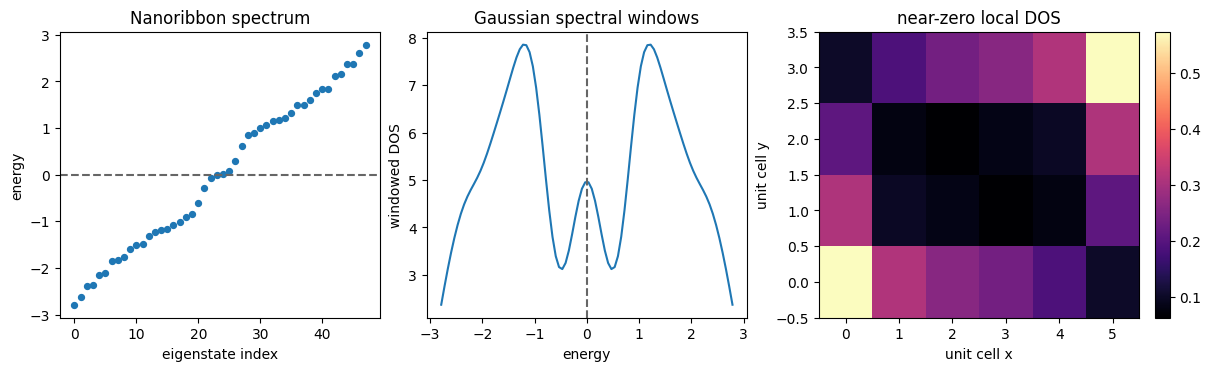
Output 1 (cell 5):
Edge Fraction [probability]: 0.6643744409979471
Output 2 (cell 9):
near_zero_window_weight: 5.032
edge_fraction_of_near_zero_ldos [probability]: 0.664
validation: passed
27_fermi_dirac_electronic_occupations.ipynb
Source: notebooks/real_examples/27_fermi_dirac_electronic_occupations.ipynb
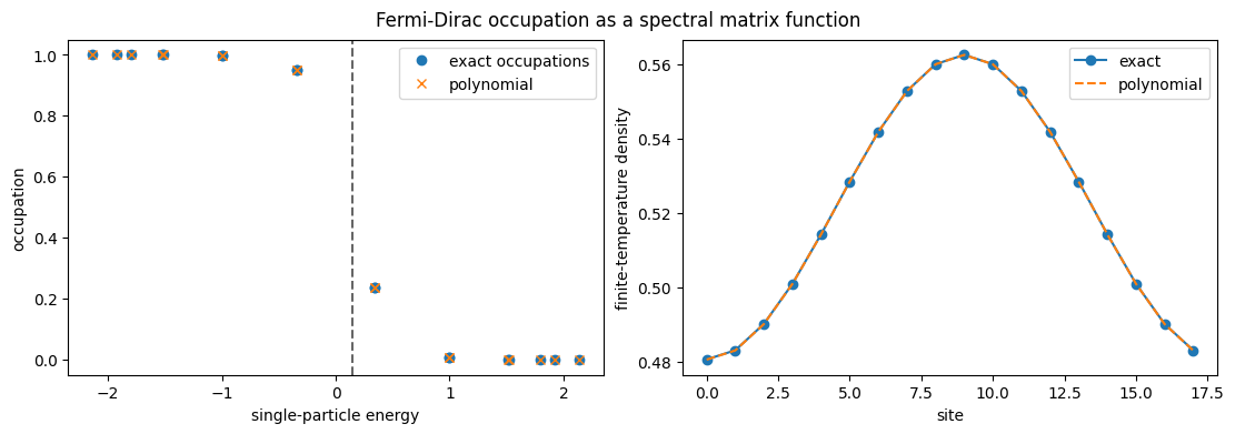
Output 1 (cell 5):
Occupation Error: 7.804084211610466e-05
Exact Particle Number [electrons]: 9.385723227081577
Polynomial Particle Number [electrons]: 9.385329756322626
Output 2 (cell 7):
relative_density_matrix_error: 0.0001
exact_particle_number [electrons]: 9.386
polynomial_particle_number [electrons]: 9.385
validation: passed
28_photonic_crystal_band_gap_filtering.ipynb
Source: notebooks/real_examples/28_photonic_crystal_band_gap_filtering.ipynb
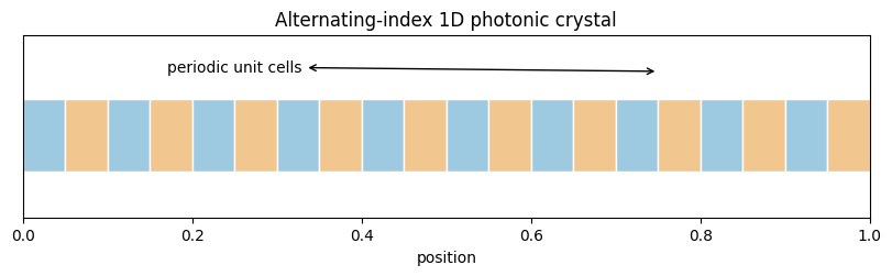
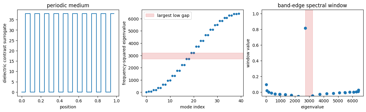
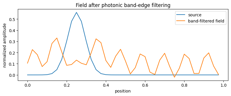
Output 1 (cell 5):
Gap Size [model frequency units]: 500.45893808166556
Target Energy [model frequency units]: 2718.4282533951346
Maximum Mode Weight: 0.8135833929662374
Output 2 (cell 10):
selected_gap_index [index]: 18
gap_size [model frequency units]: 500.459
max_window_weight: 0.814
validation: passed
29_topological_band_projector_chern_marker.ipynb
Source: notebooks/real_examples/29_topological_band_projector_chern_marker.ipynb
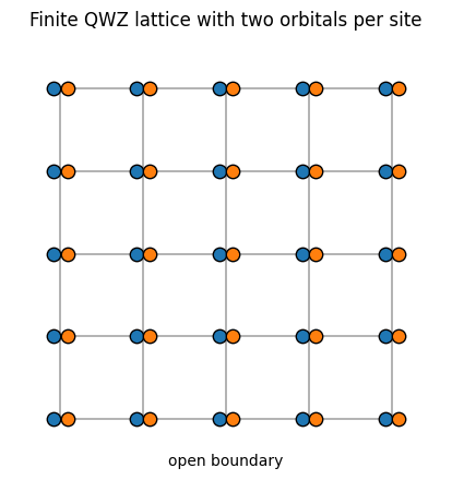
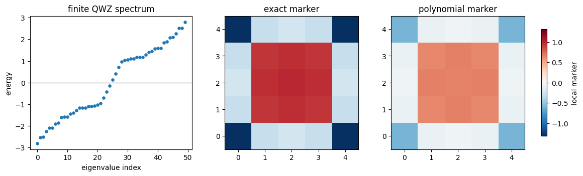
Output 1 (cell 6):
Dimension [states]: 50
Spectral range [model energy units]: (-2.800243765865765, 2.8002437658657637)
Gap around zero [model energy units]: 0.13742301418061872
Output 2 (cell 10):
Scaled gap: 0.04907537545686846
Projector relative error: 0.10636398990180881
Output 3 (cell 12):
Marker relative error: 0.45526864295151465
Bulk exact marker [Chern marker]: 0.9583268200049554
Bulk polynomial marker [Chern marker]: 0.6430191290198954
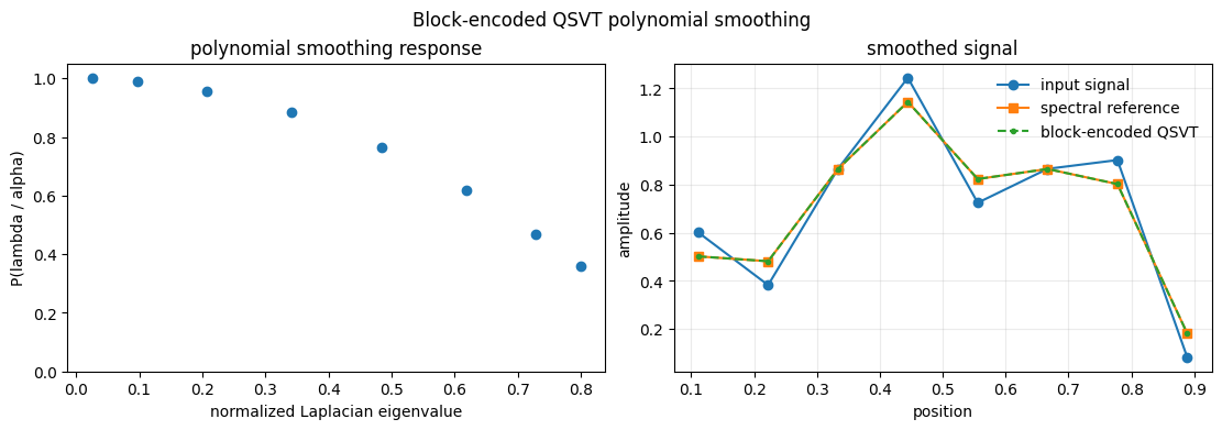
30_block_encoded_laplacian_smoothing.ipynb
Source: notebooks/real_examples/30_block_encoded_laplacian_smoothing.ipynb
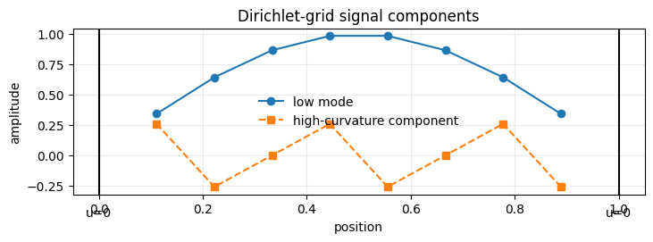
Output 1 (cell 6):
Block-Encoding Alpha: 392.788
Logical Dimension: 8
Unitary Dimension: 16
Block Error: 0.000e+00
Unitarity Error: 3.819e-15
Operator Relative Error: 1.001e-12
State Relative Error: 1.001e-12
Output 2 (cell 8):
QNode Execution Kind: pennylane-qnode-statevector-qsvt-execution
QNode Gate Types: {'StatePrep': 1, 'QSVT': 1}
QNode Logical Success Probability: 0.959851950246
QNode Real Logical Error: 9.746e-13
QNode Max Imaginary Logical Amplitude: 4.517e-02
Output 3 (cell 14):
validation: passed